
Methodology, Parameters, and Calculations
Keywords
health economics methodology, clinical trial cost analysis, medical research ROI, cost-benefit analysis healthcare, sensitivity analysis, Monte Carlo simulation, DALY calculation, pragmatic clinical trials
Overview
This appendix documents all 23 parameters used in the analysis, organized by type:
- External sources (peer-reviewed): 8
- Calculated values: 11
- Core definitions: 4
Calculated Values
Parameters derived from mathematical formulas and economic models.
Pragmatic Trial Cost Reduction Factor: 44.1x
Note📊 Details
Cost reduction factor projected for embedded pragmatic trials (traditional Phase 3 cost / pragmatic trial cost per patient)
Inputs:
- Phase 3 Cost per Patient 📊: $41,000 (95% CI: $20,000 - $120,000)
- Pragmatic Trial Cost per Patient 📊: $929 (95% CI: $97 - $3,000)
\[ \begin{gathered} k_{reduce} \\ = \frac{Cost_{P3,pt}}{Cost_{pragmatic,pt}} \\ = \frac{\$41K}{\$929} \\ = 44.1 \end{gathered} \]
✓ High confidence
Sensitivity Analysis
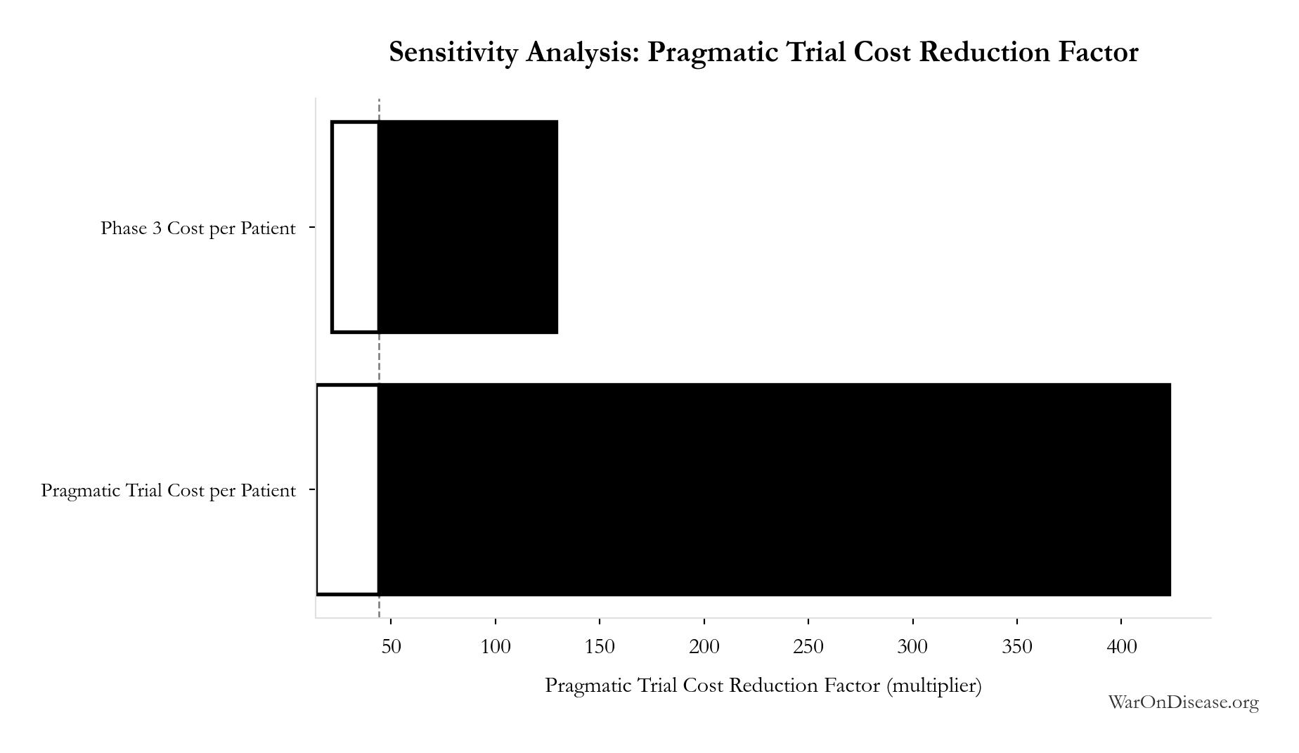
Sensitivity Indices for Pragmatic Trial Cost Reduction Factor
Regression-based sensitivity showing which inputs explain the most variance in the output.
| Input Parameter | Sensitivity Coefficient | Interpretation |
|---|---|---|
| Phase 3 Cost per Patient (USD/patient) | 0.5310 | Strong driver |
| Pragmatic Trial Cost per Patient (USD/patient) | -0.4880 | Moderate driver |
Interpretation: Standardized coefficients show the change in output (in SD units) per 1 SD change in input. Values near ±1 indicate strong influence; values exceeding ±1 may occur with correlated inputs.
Monte Carlo Distribution
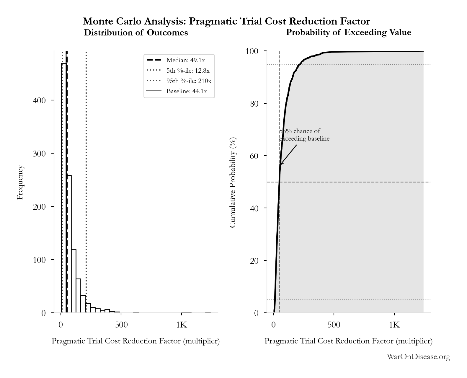
Simulation Results Summary: Pragmatic Trial Cost Reduction Factor
| Statistic | Value |
|---|---|
| Baseline (deterministic) | 44.1x |
| Mean (expected value) | 73x |
| Median (50th percentile) | 49.1x |
| Standard Deviation | 78.5x |
| 90% Range (5th-95th percentile) | [12.8x, 210x] |
The histogram shows the distribution of Pragmatic Trial Cost Reduction Factor across 10,000 Monte Carlo simulations. The CDF (right) shows the probability of the outcome exceeding any given value, which is useful for risk assessment.
Exceedance Probability
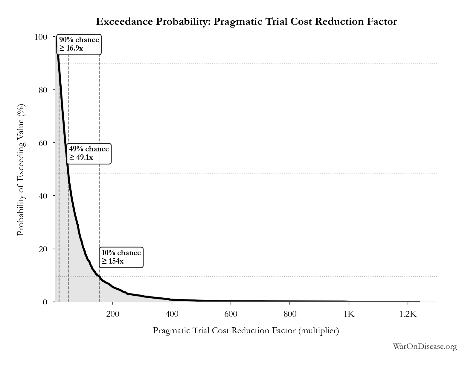
This exceedance probability chart shows the likelihood that Pragmatic Trial Cost Reduction Factor will exceed any given threshold. Higher curves indicate more favorable outcomes with greater certainty.
Diseases Without Effective Treatment: 6,650 diseases
Note📊 Details
Number of diseases without effective treatment. 95% of 7,000 rare diseases lack FDA-approved treatment (per Orphanet 2024). This represents the therapeutic search space that remains unexplored.
Inputs:
- Total Number of Rare Diseases Globally 📊: 7,000 diseases (95% CI: 6,000 diseases - 10,000 diseases)
\[ \begin{gathered} N_{untreated} \\ = N_{rare} \times 0.95 \\ = 7{,}000 \times 0.95 \\ = 6{,}650 \end{gathered} \]
Methodology:3
~ Medium confidence
Sensitivity Analysis
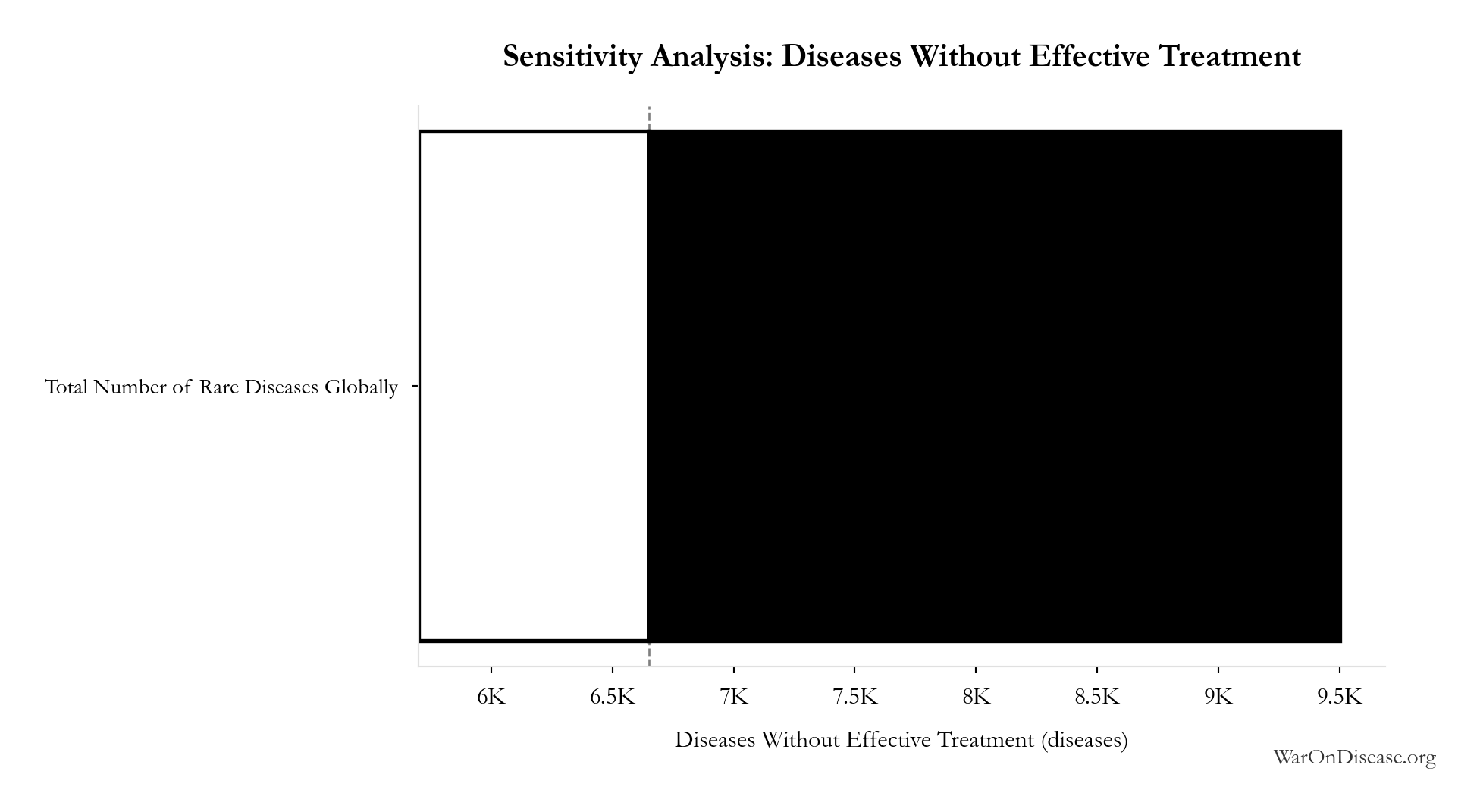
Sensitivity Indices for Diseases Without Effective Treatment
Regression-based sensitivity showing which inputs explain the most variance in the output.
| Input Parameter | Sensitivity Coefficient | Interpretation |
|---|---|---|
| Total Number of Rare Diseases Globally (diseases) | 1.0000 | Strong driver |
Interpretation: Standardized coefficients show the change in output (in SD units) per 1 SD change in input. Values near ±1 indicate strong influence; values exceeding ±1 may occur with correlated inputs.
Monte Carlo Distribution
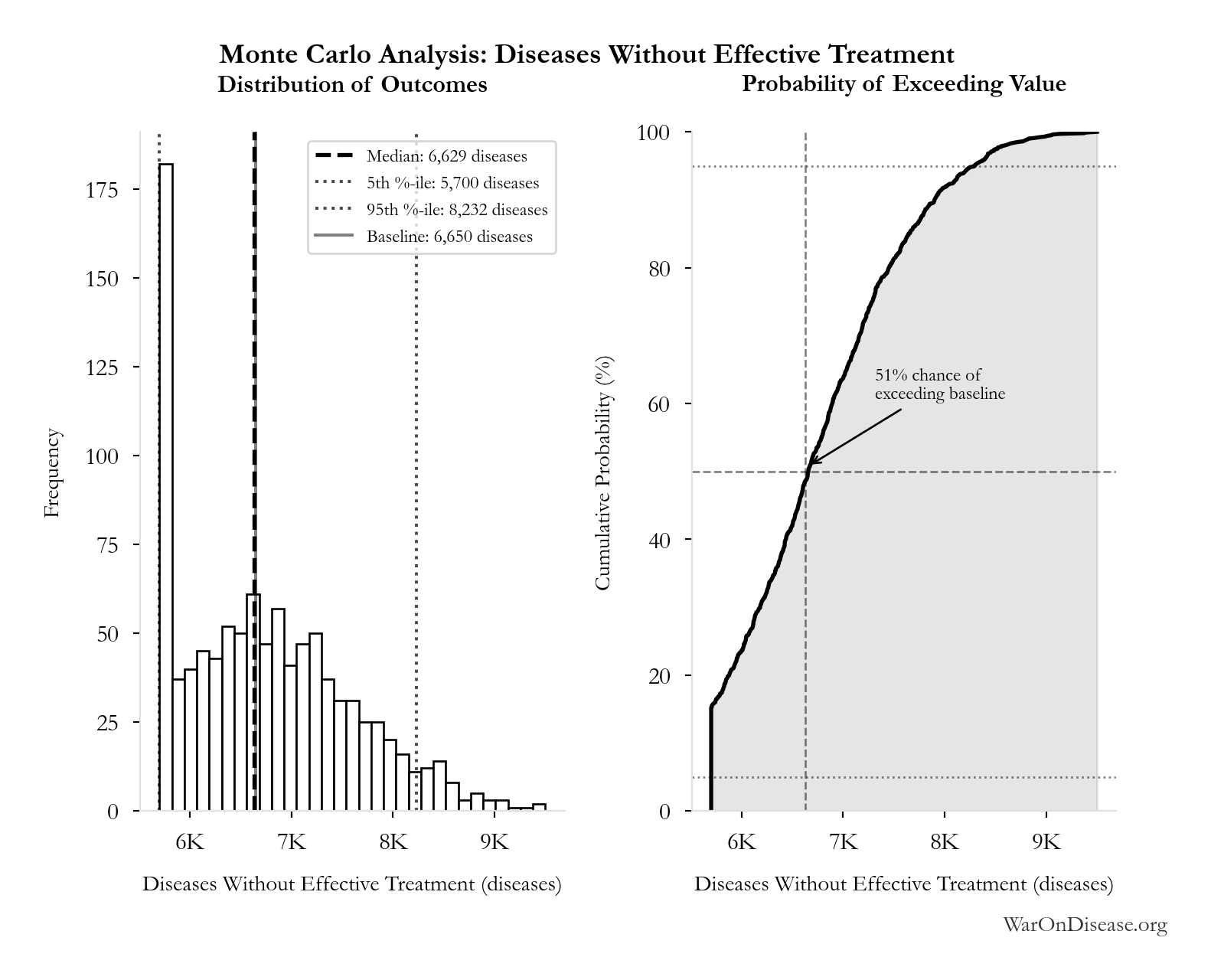
Simulation Results Summary: Diseases Without Effective Treatment
| Statistic | Value |
|---|---|
| Baseline (deterministic) | 6,650 |
| Mean (expected value) | 6,718 |
| Median (50th percentile) | 6,629 |
| Standard Deviation | 827 |
| 90% Range (5th-95th percentile) | [5,700, 8,232] |
The histogram shows the distribution of Diseases Without Effective Treatment across 10,000 Monte Carlo simulations. The CDF (right) shows the probability of the outcome exceeding any given value, which is useful for risk assessment.
Exceedance Probability
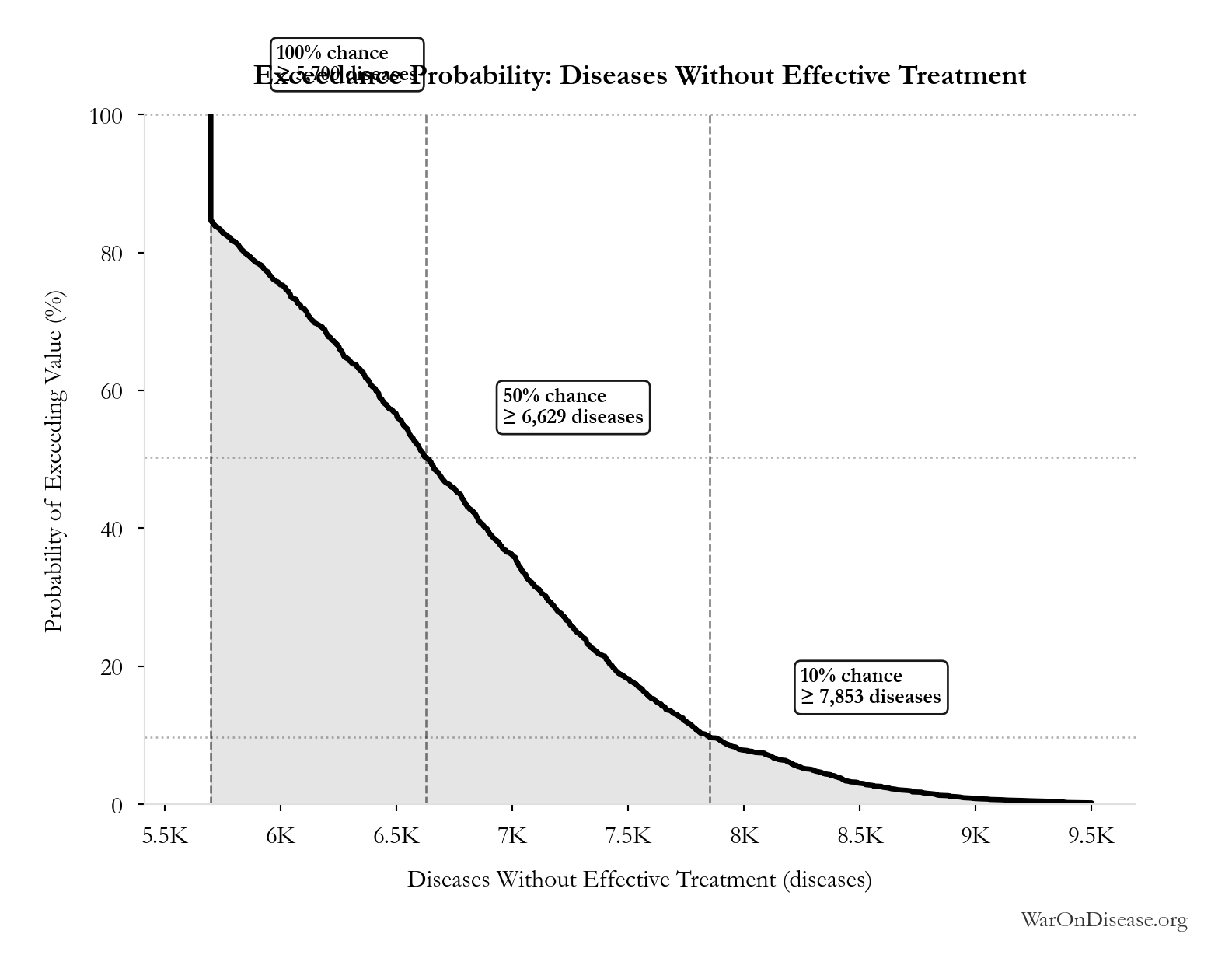
This exceedance probability chart shows the likelihood that Diseases Without Effective Treatment will exceed any given threshold. Higher curves indicate more favorable outcomes with greater certainty.
Universal Right to Try with Evidence Philanthropic Cost per DALY: $0.000134
Note📊 Details
Conditional philanthropic cost per DALY if all 50 states adopt, a mature pooled pragmatic-trial system operates under applicable federal authorization, and the modeled treatment-discovery acceleration occurs. The numerator includes the 50-state campaign and ten-year registry launch costs, excludes patient or payer spending on treatment delivery, trial-site services, and permitted study costs, and assumes center assessments fund the registry thereafter. The denominator counts the global treatment schedule shift once.
Inputs:
- Universal Right to Try with Evidence Philanthropic Cost: $65 million (95% CI: $25 million - $200 million)
- DALYs Averted from Universal Right to Try with Evidence 🔢: 483 billion DALYs
\[ \begin{gathered} Cost_{RTT,DALY} \\ = \frac{C_{RTT}}{DALYs_{RTT}} \\ = \frac{\$65M}{483B} \\ = \$0.000134 \end{gathered} \] where: \[ \begin{gathered} DALYs_{RTT} \\ = DALYs_{global,ann} \times Pct_{avoid,DALY} \times T_{accel,RTT} \\ = 2.88B \times 92.6\% \times 181 \\ = 483B \end{gathered} \] where: \[ \begin{gathered} T_{accel,RTT} \\ = T_{first,SQ} \times \left(1 - \frac{1}{k_{RTT}}\right) \\ = 222 \times \left(1 - \frac{1}{5.48}\right) \\ = 181 \end{gathered} \] where: \[ \begin{gathered} T_{first,SQ} \\ = T_{queue,SQ} \times 0.5 \\ = 443 \times 0.5 \\ = 222 \end{gathered} \] where: \[ \begin{gathered} T_{queue,SQ} \\ = \frac{N_{untreated}}{Treatments_{new,ann}} \\ = \frac{6{,}650}{15} \\ = 443 \end{gathered} \] where: \[ \begin{gathered} N_{untreated} \\ = N_{rare} \times 0.95 \\ = 7{,}000 \times 0.95 \\ = 6{,}650 \end{gathered} \] ? Low confidence
Sensitivity Analysis
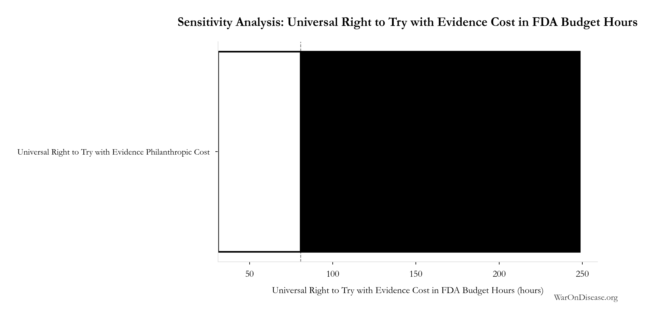
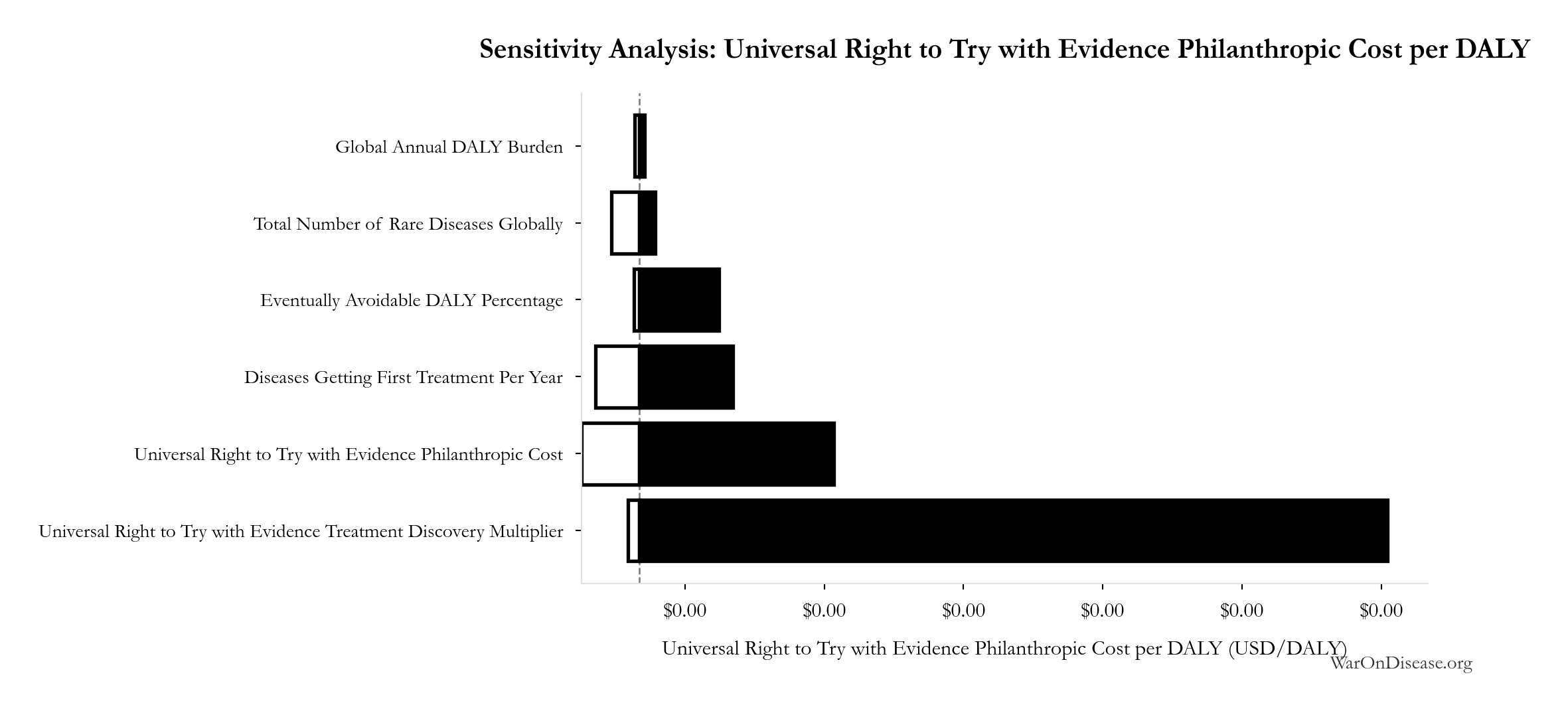
Sensitivity Indices for Universal Right to Try with Evidence Philanthropic Cost per DALY
Regression-based sensitivity showing which inputs explain the most variance in the output.
| Input Parameter | Sensitivity Coefficient | Interpretation |
|---|---|---|
| Universal Right to Try with Evidence Philanthropic Cost (USD) | 0.5604 | Strong driver |
| DALYs Averted from Universal Right to Try with Evidence (DALYs) | -0.4511 | Moderate driver |
Interpretation: Standardized coefficients show the change in output (in SD units) per 1 SD change in input. Values near ±1 indicate strong influence; values exceeding ±1 may occur with correlated inputs.
Monte Carlo Distribution
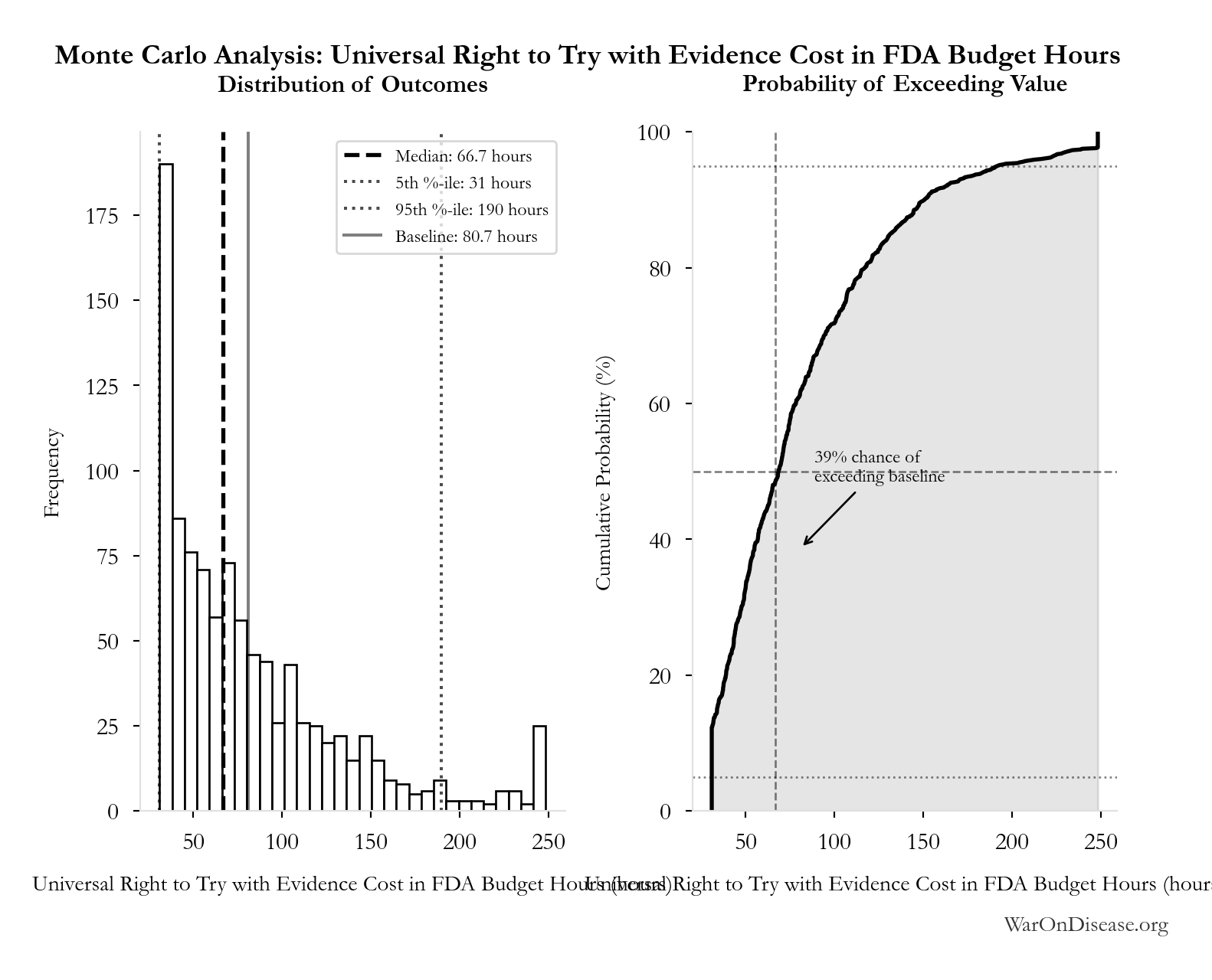
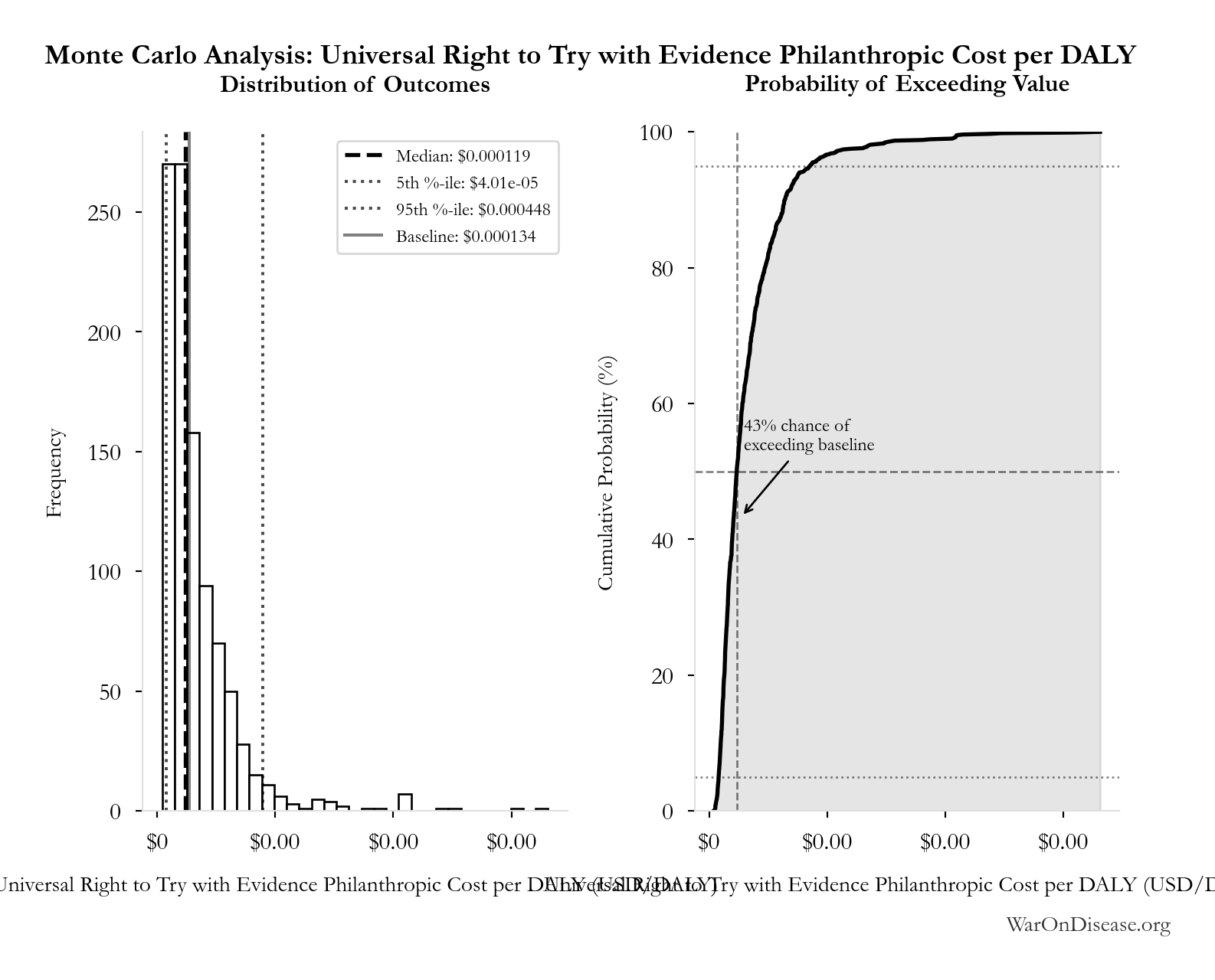
Simulation Results Summary: Universal Right to Try with Evidence Philanthropic Cost per DALY
| Statistic | Value |
|---|---|
| Baseline (deterministic) | $0.000134 |
| Mean (expected value) | $0.000171 |
| Median (50th percentile) | $0.000119 |
| Standard Deviation | $0.000192 |
| 90% Range (5th-95th percentile) | [$4.01e-05, $0.000448] |
The histogram shows the distribution of Universal Right to Try with Evidence Philanthropic Cost per DALY across 10,000 Monte Carlo simulations. The CDF (right) shows the probability of the outcome exceeding any given value, which is useful for risk assessment.
Exceedance Probability
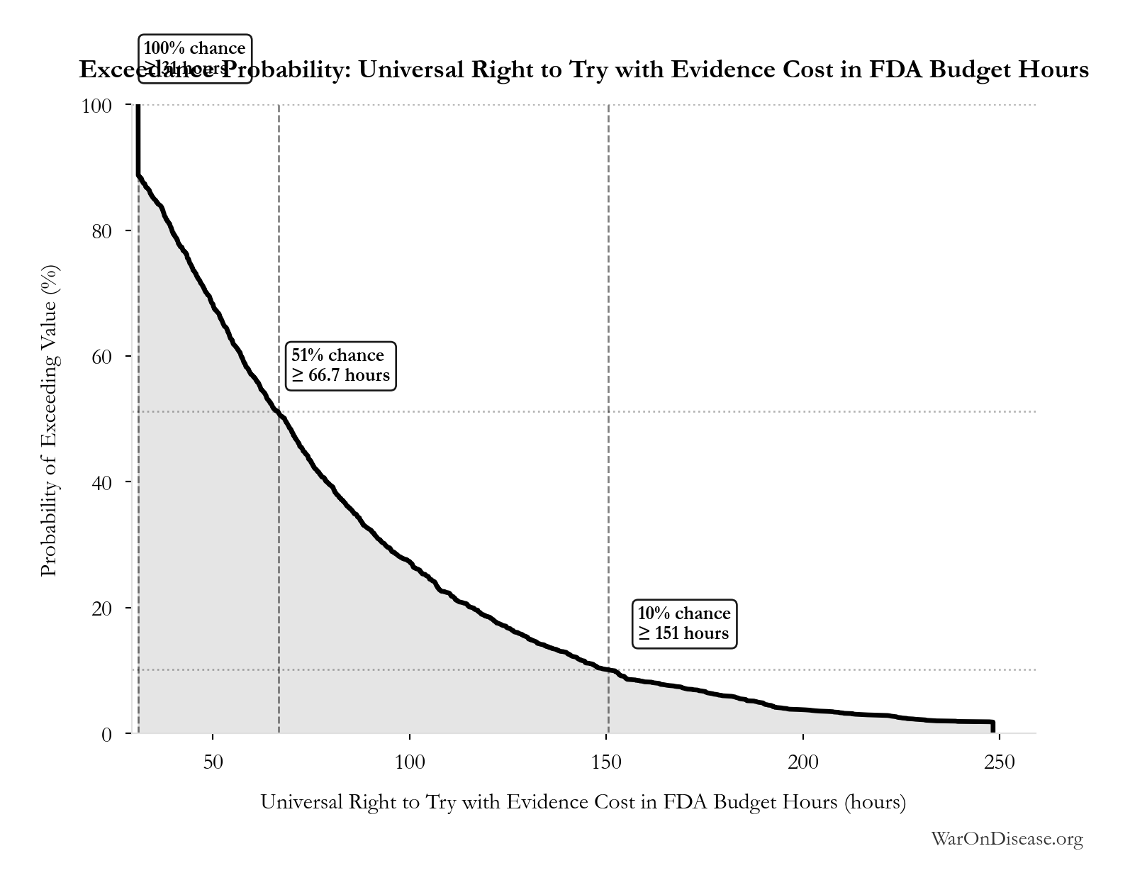
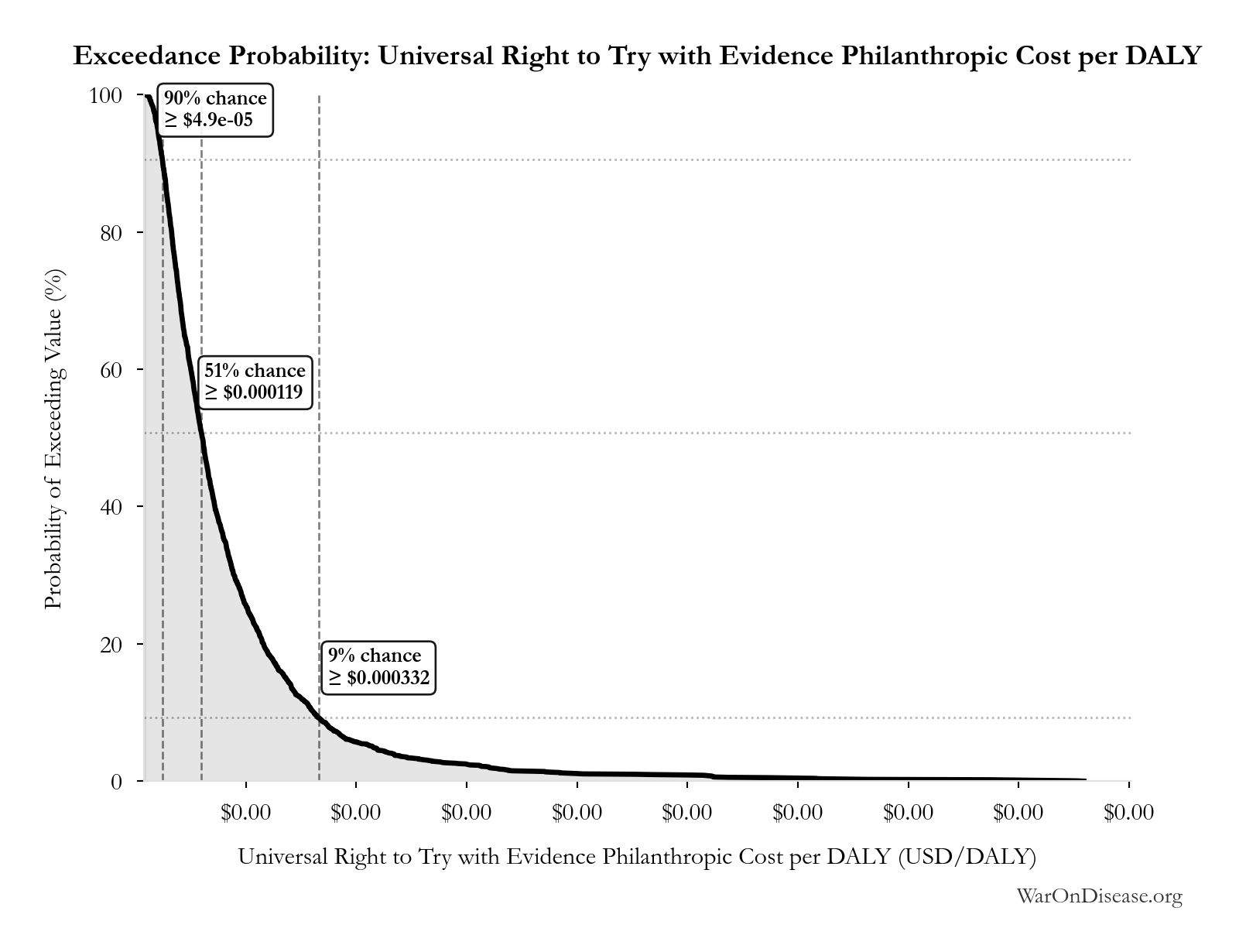
This exceedance probability chart shows the likelihood that Universal Right to Try with Evidence Philanthropic Cost per DALY will exceed any given threshold. Higher curves indicate more favorable outcomes with greater certainty.
Universal Right to Try with Evidence Philanthropic Cost per Life Saved: $0.00707
Note📊 Details
Conditional philanthropic cost per modeled premature death prevented if all 50 states adopt, a mature pooled pragmatic-trial system operates, and the modeled treatment-discovery acceleration occurs. This uses the same campaign and registry numerator as the cost-per-DALY estimate.
Inputs:
- Universal Right to Try with Evidence Philanthropic Cost: $65 million (95% CI: $25 million - $200 million)
- Lives Saved from Universal Right to Try with Evidence 🔢: 9.19 billion deaths
\[ \begin{gathered} Cost_{RTT,life} \\ = \frac{C_{RTT}}{Lives_{RTT}} \\ = \frac{\$65M}{9.19B} \\ = \$0.00707 \end{gathered} \] where: \[ \begin{gathered} Lives_{RTT} \\ = Deaths_{disease,daily} \times Pct_{avoid,death} \times T_{accel,RTT} \times 365 \\ = 150{,}000 \times 92.6\% \times 181 \times 365 \\ = 9.19B \end{gathered} \] where: \[ \begin{gathered} T_{accel,RTT} \\ = T_{first,SQ} \times \left(1 - \frac{1}{k_{RTT}}\right) \\ = 222 \times \left(1 - \frac{1}{5.48}\right) \\ = 181 \end{gathered} \] where: \[ \begin{gathered} T_{first,SQ} \\ = T_{queue,SQ} \times 0.5 \\ = 443 \times 0.5 \\ = 222 \end{gathered} \] where: \[ \begin{gathered} T_{queue,SQ} \\ = \frac{N_{untreated}}{Treatments_{new,ann}} \\ = \frac{6{,}650}{15} \\ = 443 \end{gathered} \] where: \[ \begin{gathered} N_{untreated} \\ = N_{rare} \times 0.95 \\ = 7{,}000 \times 0.95 \\ = 6{,}650 \end{gathered} \] ? Low confidence
Sensitivity Analysis
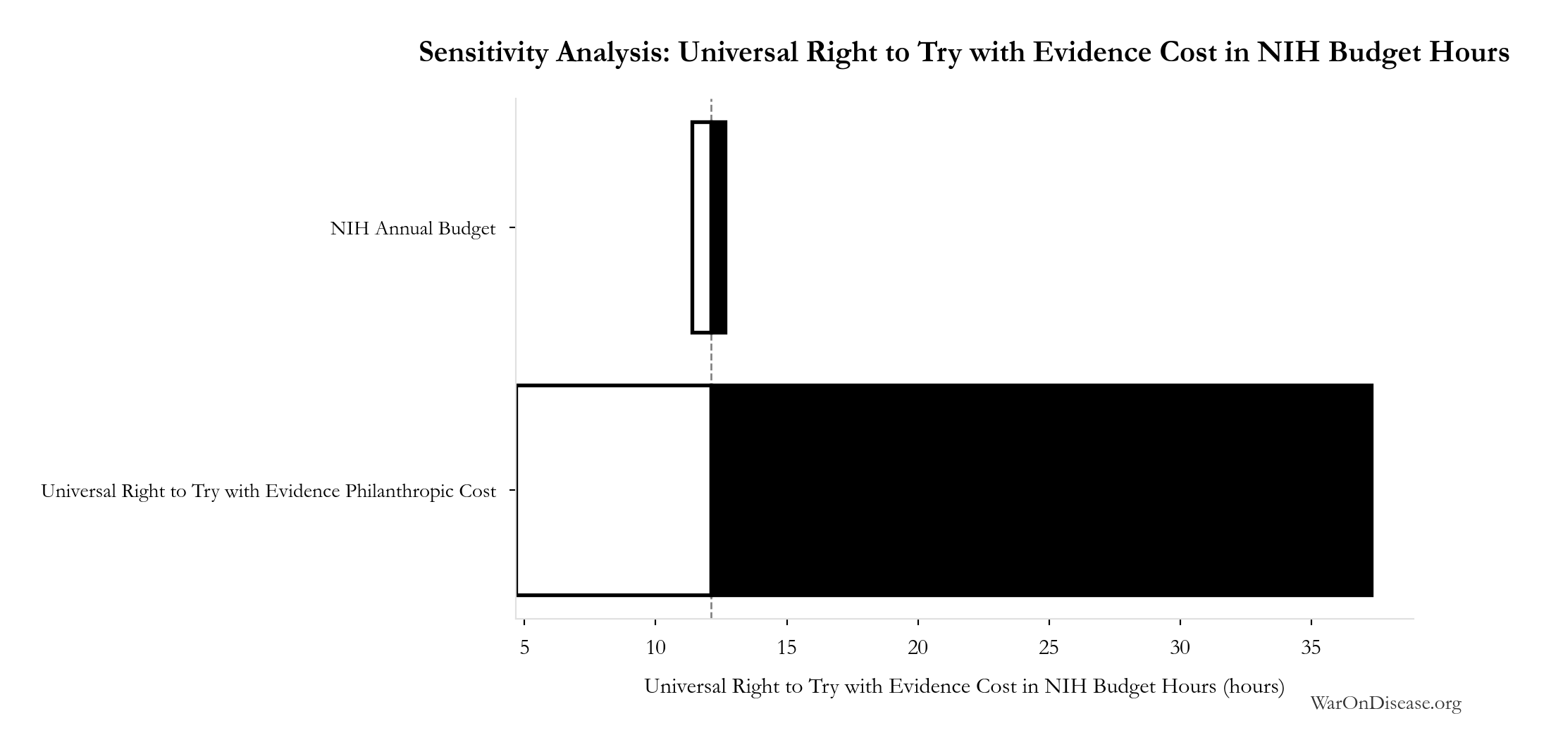
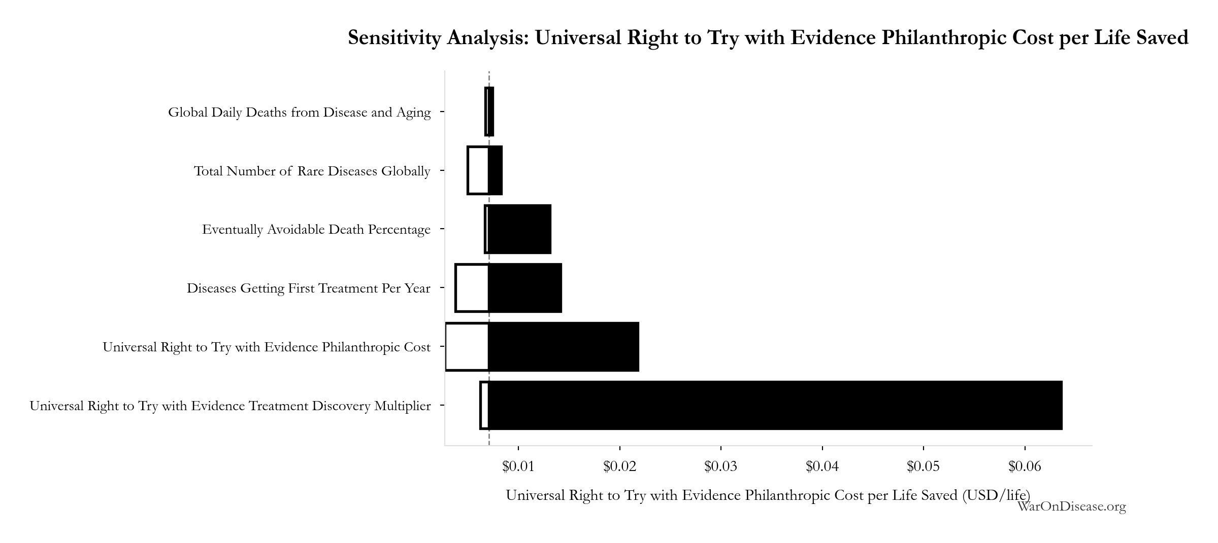
Sensitivity Indices for Universal Right to Try with Evidence Philanthropic Cost per Life Saved
Regression-based sensitivity showing which inputs explain the most variance in the output.
| Input Parameter | Sensitivity Coefficient | Interpretation |
|---|---|---|
| Universal Right to Try with Evidence Philanthropic Cost (USD) | 0.5418 | Strong driver |
| Lives Saved from Universal Right to Try with Evidence (deaths) | -0.4450 | Moderate driver |
Interpretation: Standardized coefficients show the change in output (in SD units) per 1 SD change in input. Values near ±1 indicate strong influence; values exceeding ±1 may occur with correlated inputs.
Monte Carlo Distribution
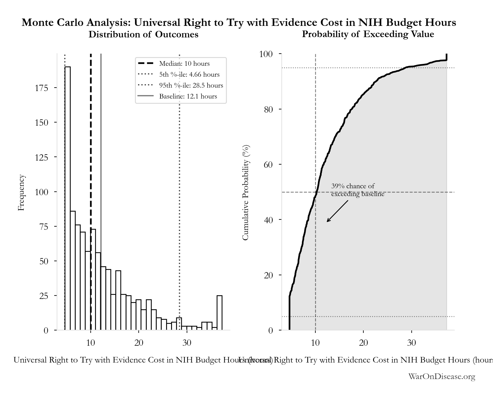
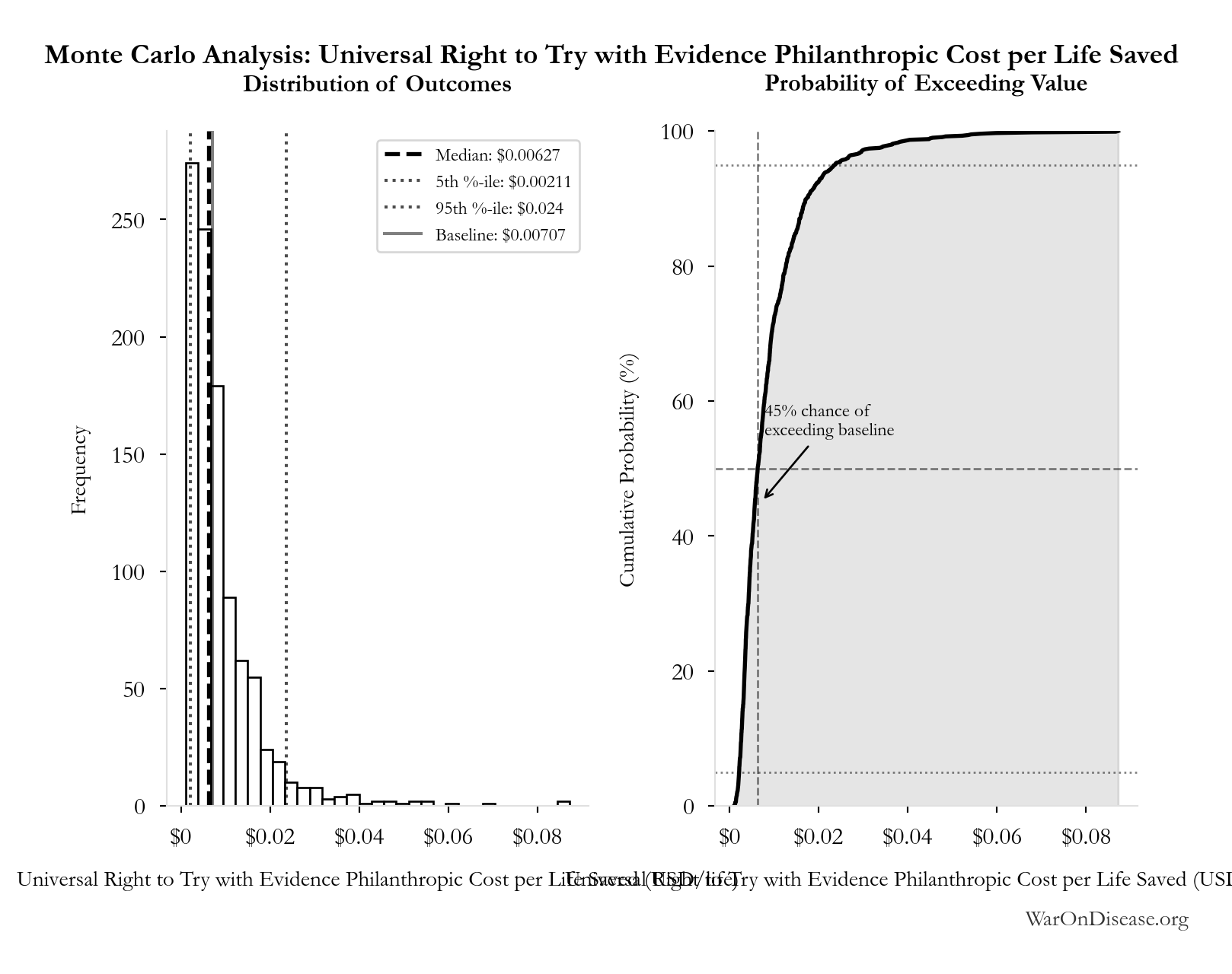
Simulation Results Summary: Universal Right to Try with Evidence Philanthropic Cost per Life Saved
| Statistic | Value |
|---|---|
| Baseline (deterministic) | $0.00707 |
| Mean (expected value) | $0.00907 |
| Median (50th percentile) | $0.00627 |
| Standard Deviation | $0.01 |
| 90% Range (5th-95th percentile) | [$0.00211, $0.024] |
The histogram shows the distribution of Universal Right to Try with Evidence Philanthropic Cost per Life Saved across 10,000 Monte Carlo simulations. The CDF (right) shows the probability of the outcome exceeding any given value, which is useful for risk assessment.
Exceedance Probability
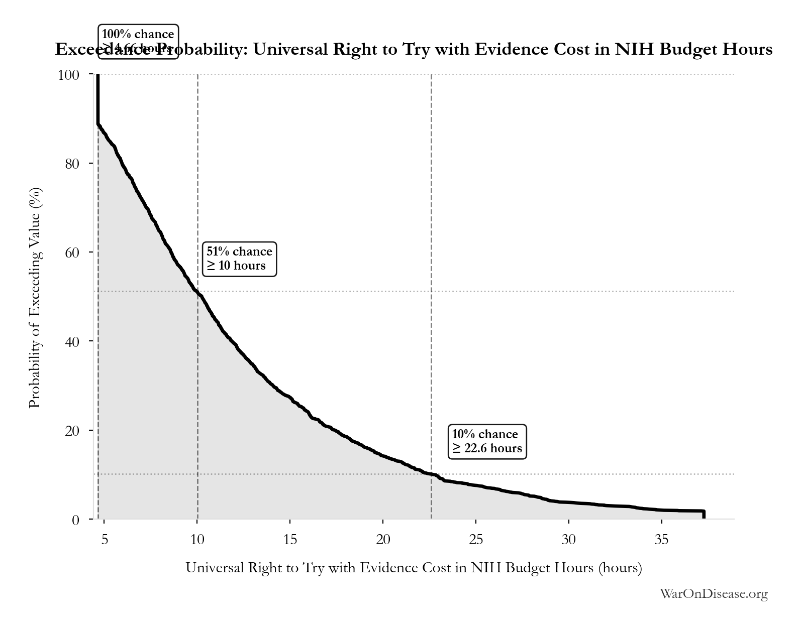
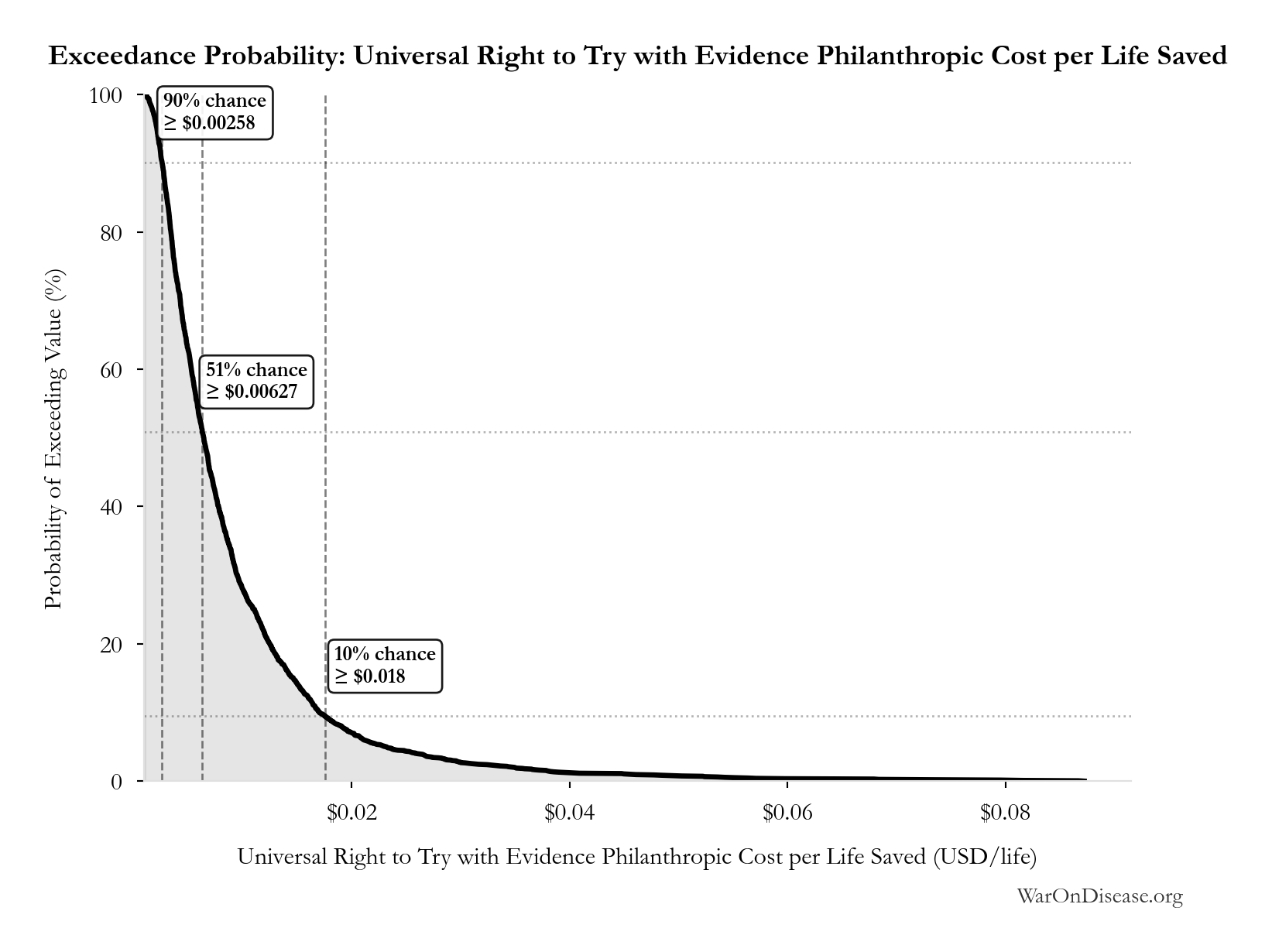
This exceedance probability chart shows the likelihood that Universal Right to Try with Evidence Philanthropic Cost per Life Saved will exceed any given threshold. Higher curves indicate more favorable outcomes with greater certainty.
DALYs Averted from Universal Right to Try with Evidence: 483 billion DALYs
Note📊 Details
Conditional lifetime DALYs averted by shifting the global treatment-discovery schedule forward. By design, this applies the therapeutic-discovery timeline proxy to the eventually avoidable burden of all global diseases and aging-related degeneration. It is a schedule-shift calculation across future generations, not an observed epidemiological forecast.
Inputs:
- Global Annual DALY Burden 📊: 2.88 billion DALYs/year (SE: ±150 million DALYs/year)
- Eventually Avoidable DALY Percentage: 92.6% (95% CI: 50% - 98%)
- Average Treatment Acceleration from Universal Right to Try with Evidence 🔢: 181 years
\[ \begin{gathered} DALYs_{RTT} \\ = DALYs_{global,ann} \times Pct_{avoid,DALY} \times T_{accel,RTT} \\ = 2.88B \times 92.6\% \times 181 \\ = 483B \end{gathered} \] where: \[ \begin{gathered} T_{accel,RTT} \\ = T_{first,SQ} \times \left(1 - \frac{1}{k_{RTT}}\right) \\ = 222 \times \left(1 - \frac{1}{5.48}\right) \\ = 181 \end{gathered} \] where: \[ \begin{gathered} T_{first,SQ} \\ = T_{queue,SQ} \times 0.5 \\ = 443 \times 0.5 \\ = 222 \end{gathered} \] where: \[ \begin{gathered} T_{queue,SQ} \\ = \frac{N_{untreated}}{Treatments_{new,ann}} \\ = \frac{6{,}650}{15} \\ = 443 \end{gathered} \] where: \[ \begin{gathered} N_{untreated} \\ = N_{rare} \times 0.95 \\ = 7{,}000 \times 0.95 \\ = 6{,}650 \end{gathered} \] ? Low confidence
Sensitivity Analysis
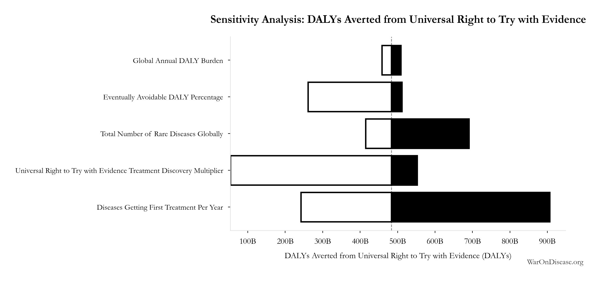
Sensitivity Indices for DALYs Averted from Universal Right to Try with Evidence
Regression-based sensitivity showing which inputs explain the most variance in the output.
| Input Parameter | Sensitivity Coefficient | Interpretation |
|---|---|---|
| Average Treatment Acceleration from Universal Right to Try with Evidence (years) | 0.9488 | Strong driver |
| Eventually Avoidable DALY Percentage (percentage) | 0.2682 | Weak driver |
| Global Annual DALY Burden (DALYs/year) | 0.1167 | Weak driver |
Interpretation: Standardized coefficients show the change in output (in SD units) per 1 SD change in input. Values near ±1 indicate strong influence; values exceeding ±1 may occur with correlated inputs.
Monte Carlo Distribution
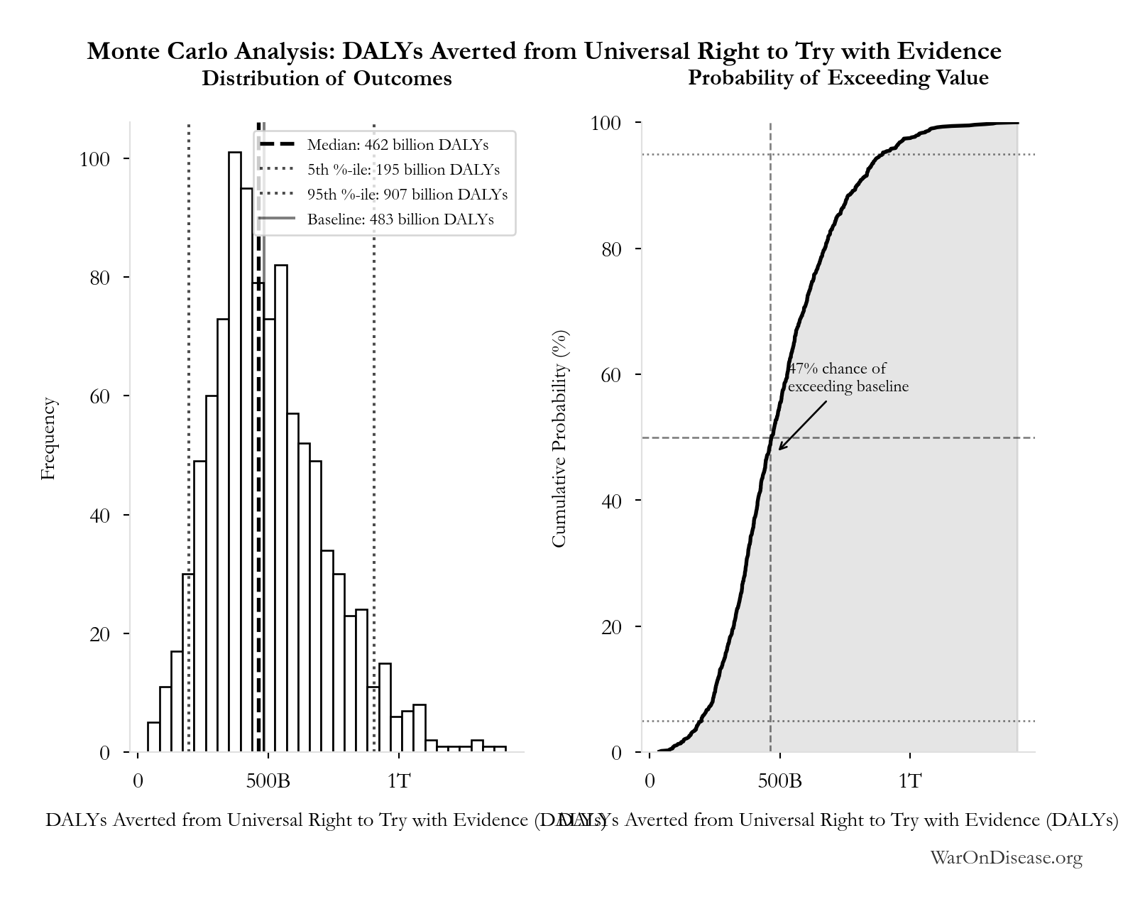
Simulation Results Summary: DALYs Averted from Universal Right to Try with Evidence
| Statistic | Value |
|---|---|
| Baseline (deterministic) | 483 billion |
| Mean (expected value) | 495 billion |
| Median (50th percentile) | 462 billion |
| Standard Deviation | 217 billion |
| 90% Range (5th-95th percentile) | [195 billion, 907 billion] |
The histogram shows the distribution of DALYs Averted from Universal Right to Try with Evidence across 10,000 Monte Carlo simulations. The CDF (right) shows the probability of the outcome exceeding any given value, which is useful for risk assessment.
Exceedance Probability
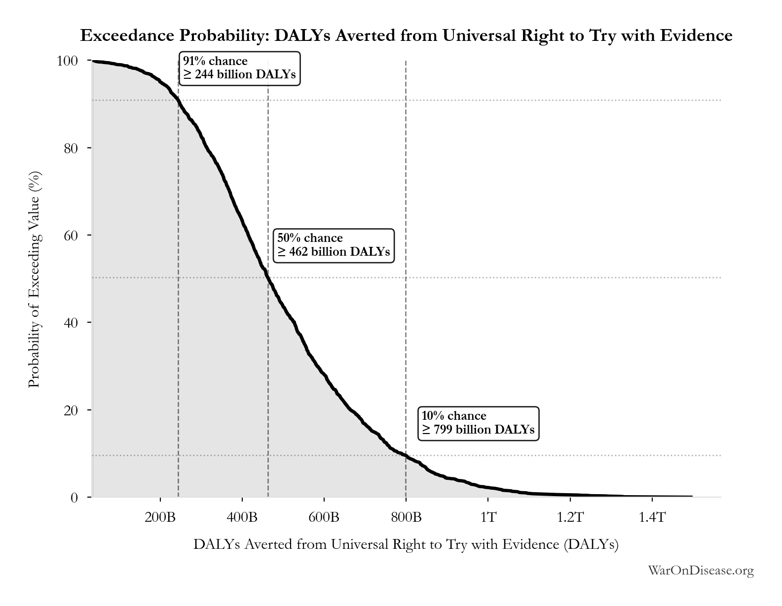
This exceedance probability chart shows the likelihood that DALYs Averted from Universal Right to Try with Evidence will exceed any given threshold. Higher curves indicate more favorable outcomes with greater certainty.
Lives Saved from Universal Right to Try with Evidence: 9.19 billion deaths
Note📊 Details
Conditional cumulative premature deaths from global diseases and aging prevented across future generations by shifting the treatment-discovery schedule forward. The total can exceed the current population because it sums deaths prevented over the full acceleration period.
Inputs:
- Global Daily Deaths from Disease and Aging 📊: 150 thousand deaths/day (SE: ±7,500 deaths/day)
- Eventually Avoidable Death Percentage: 92.6% (95% CI: 50% - 98%)
- Average Treatment Acceleration from Universal Right to Try with Evidence 🔢: 181 years
\[ \begin{gathered} Lives_{RTT} \\ = Deaths_{disease,daily} \times Pct_{avoid,death} \times T_{accel,RTT} \times 365 \\ = 150{,}000 \times 92.6\% \times 181 \times 365 \\ = 9.19B \end{gathered} \] where: \[ \begin{gathered} T_{accel,RTT} \\ = T_{first,SQ} \times \left(1 - \frac{1}{k_{RTT}}\right) \\ = 222 \times \left(1 - \frac{1}{5.48}\right) \\ = 181 \end{gathered} \] where: \[ \begin{gathered} T_{first,SQ} \\ = T_{queue,SQ} \times 0.5 \\ = 443 \times 0.5 \\ = 222 \end{gathered} \] where: \[ \begin{gathered} T_{queue,SQ} \\ = \frac{N_{untreated}}{Treatments_{new,ann}} \\ = \frac{6{,}650}{15} \\ = 443 \end{gathered} \] where: \[ \begin{gathered} N_{untreated} \\ = N_{rare} \times 0.95 \\ = 7{,}000 \times 0.95 \\ = 6{,}650 \end{gathered} \] ? Low confidence
Sensitivity Analysis
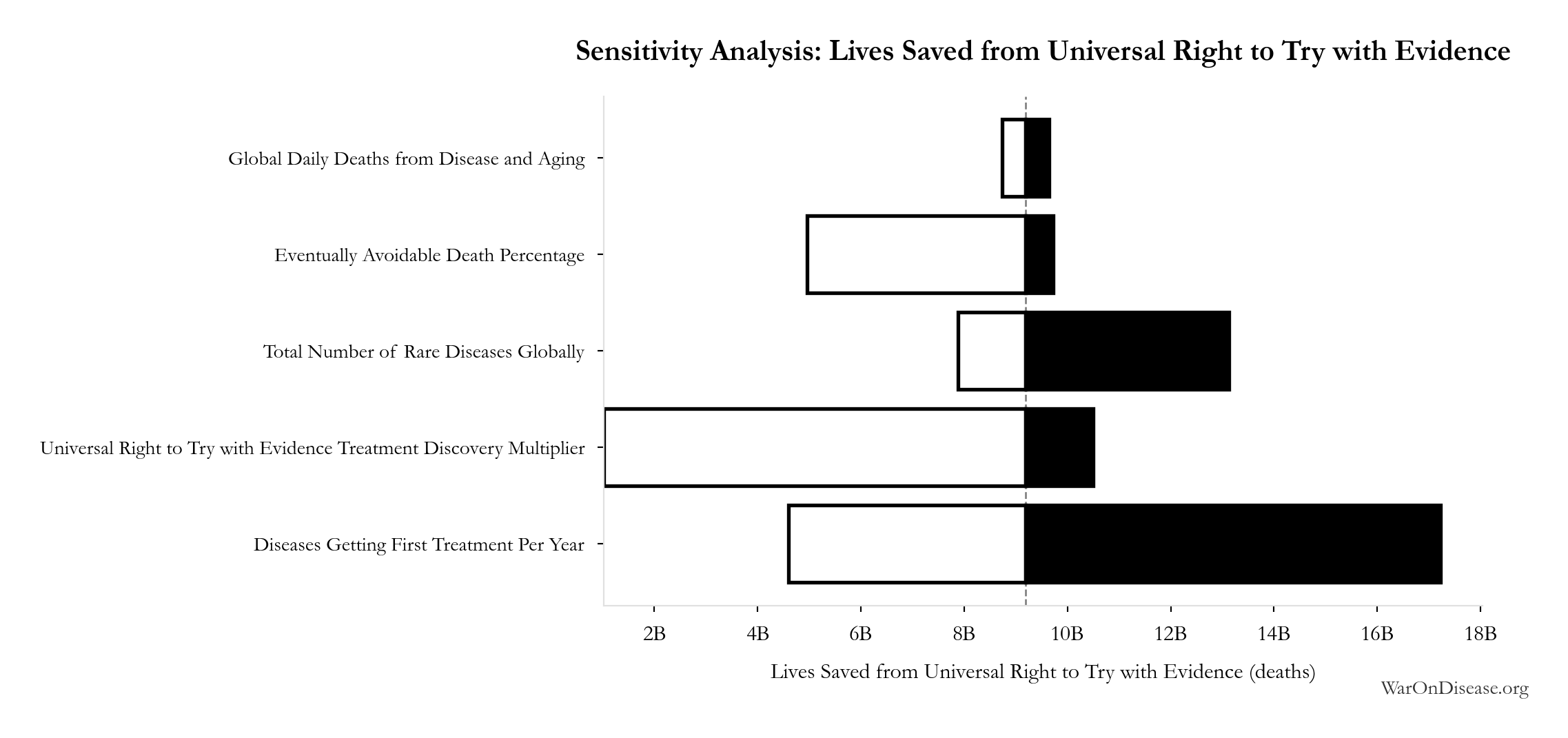
Sensitivity Indices for Lives Saved from Universal Right to Try with Evidence
Regression-based sensitivity showing which inputs explain the most variance in the output.
| Input Parameter | Sensitivity Coefficient | Interpretation |
|---|---|---|
| Average Treatment Acceleration from Universal Right to Try with Evidence (years) | 0.9436 | Strong driver |
| Eventually Avoidable Death Percentage (percentage) | 0.2710 | Weak driver |
| Global Daily Deaths from Disease and Aging (deaths/day) | 0.1115 | Weak driver |
Interpretation: Standardized coefficients show the change in output (in SD units) per 1 SD change in input. Values near ±1 indicate strong influence; values exceeding ±1 may occur with correlated inputs.
Monte Carlo Distribution
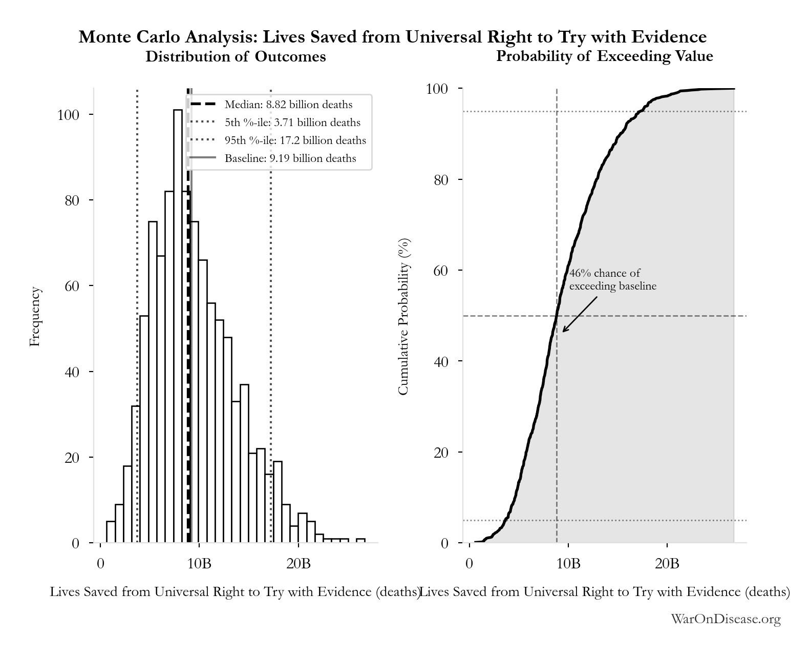
Simulation Results Summary: Lives Saved from Universal Right to Try with Evidence
| Statistic | Value |
|---|---|
| Baseline (deterministic) | 9.19 billion |
| Mean (expected value) | 9.4 billion |
| Median (50th percentile) | 8.82 billion |
| Standard Deviation | 4.13 billion |
| 90% Range (5th-95th percentile) | [3.71 billion, 17.2 billion] |
The histogram shows the distribution of Lives Saved from Universal Right to Try with Evidence across 10,000 Monte Carlo simulations. The CDF (right) shows the probability of the outcome exceeding any given value, which is useful for risk assessment.
Exceedance Probability
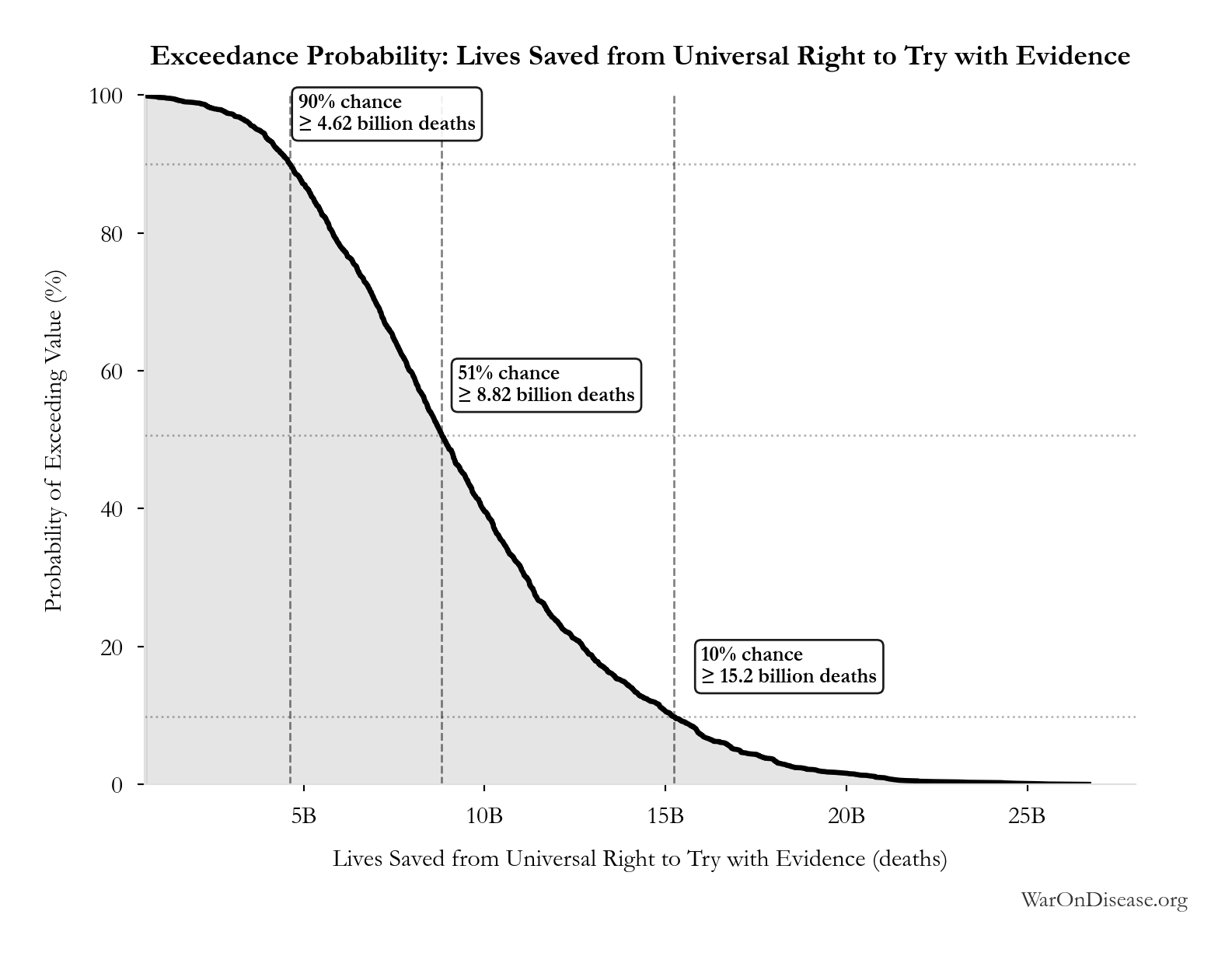
This exceedance probability chart shows the likelihood that Lives Saved from Universal Right to Try with Evidence will exceed any given threshold. Higher curves indicate more favorable outcomes with greater certainty.
Disability-Equivalent Suffering Hours Prevented by Universal Right to Try with Evidence: 1.65 quadrillion hours
Note📊 Details
Conditional disability-equivalent hours prevented by the treatment schedule shift. Converts the years-lived-with-disability share of DALYs into hours; it does not claim every hour is an hour of conscious pain.
Inputs:
- DALYs Averted from Universal Right to Try with Evidence 🔢: 483 billion DALYs
- YLD Proportion of Total DALYs 📊: 0.39 proportion (SE: ±0.03 proportion)
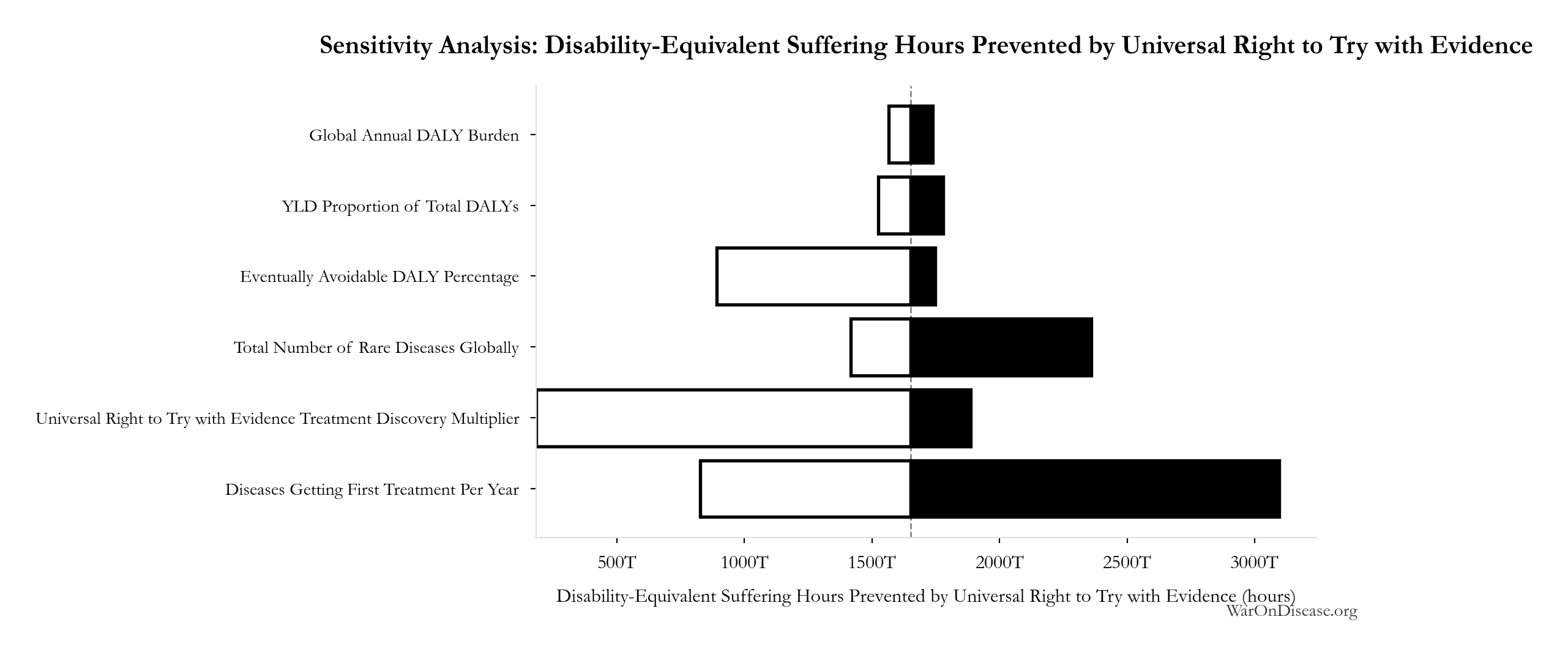
\[ \begin{gathered} Hours_{suffer,RTT} \\ = DALYs_{RTT} \times Pct_{YLD} \times 8760 \\ = 483B \times 0.39 \times 8760 \\ = 1650T \end{gathered} \] where: \[ \begin{gathered} DALYs_{RTT} \\ = DALYs_{global,ann} \times Pct_{avoid,DALY} \times T_{accel,RTT} \\ = 2.88B \times 92.6\% \times 181 \\ = 483B \end{gathered} \] where: \[ \begin{gathered} T_{accel,RTT} \\ = T_{first,SQ} \times \left(1 - \frac{1}{k_{RTT}}\right) \\ = 222 \times \left(1 - \frac{1}{5.48}\right) \\ = 181 \end{gathered} \] where: \[ \begin{gathered} T_{first,SQ} \\ = T_{queue,SQ} \times 0.5 \\ = 443 \times 0.5 \\ = 222 \end{gathered} \] where: \[ \begin{gathered} T_{queue,SQ} \\ = \frac{N_{untreated}}{Treatments_{new,ann}} \\ = \frac{6{,}650}{15} \\ = 443 \end{gathered} \] where: \[ \begin{gathered} N_{untreated} \\ = N_{rare} \times 0.95 \\ = 7{,}000 \times 0.95 \\ = 6{,}650 \end{gathered} \] ? Low confidence
Sensitivity Analysis
Sensitivity Indices for Disability-Equivalent Suffering Hours Prevented by Universal Right to Try with Evidence
Regression-based sensitivity showing which inputs explain the most variance in the output.
| Input Parameter | Sensitivity Coefficient | Interpretation |
|---|---|---|
| DALYs Averted from Universal Right to Try with Evidence (DALYs) | 0.9822 | Strong driver |
| YLD Proportion of Total DALYs (proportion) | 0.1721 | Weak driver |
Interpretation: Standardized coefficients show the change in output (in SD units) per 1 SD change in input. Values near ±1 indicate strong influence; values exceeding ±1 may occur with correlated inputs.
Monte Carlo Distribution
Simulation Results Summary: Disability-Equivalent Suffering Hours Prevented by Universal Right to Try with Evidence
| Statistic | Value |
|---|---|
| Baseline (deterministic) | 1.65 quadrillion |
| Mean (expected value) | 1.69 quadrillion |
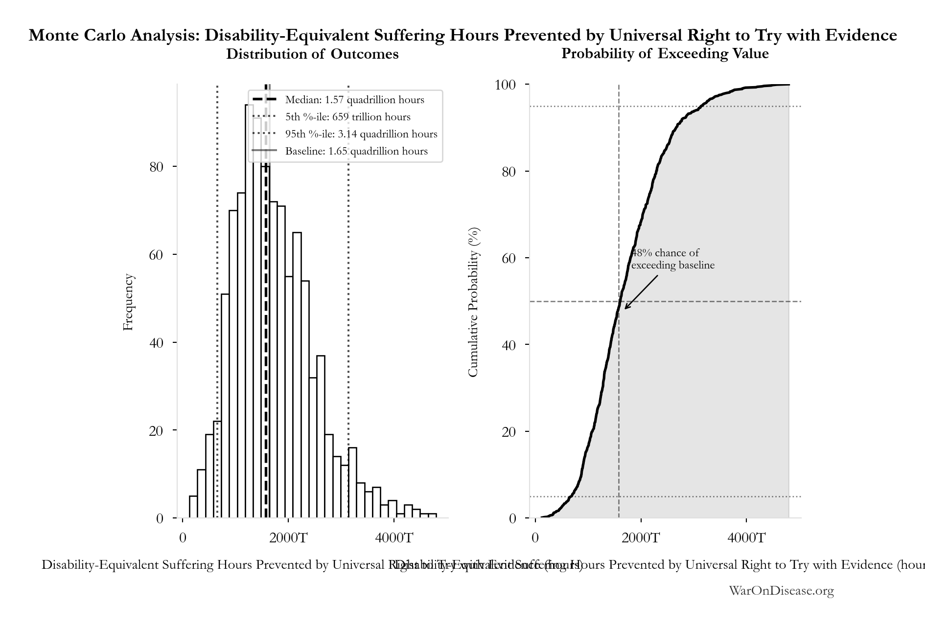
| Median (50th percentile) | 1.57 quadrillion |
| Standard Deviation | 756 trillion |
| 90% Range (5th-95th percentile) | [659 trillion, 3.14 quadrillion] |
The histogram shows the distribution of Disability-Equivalent Suffering Hours Prevented by Universal Right to Try with Evidence across 10,000 Monte Carlo simulations. The CDF (right) shows the probability of the outcome exceeding any given value, which is useful for risk assessment.
Exceedance Probability
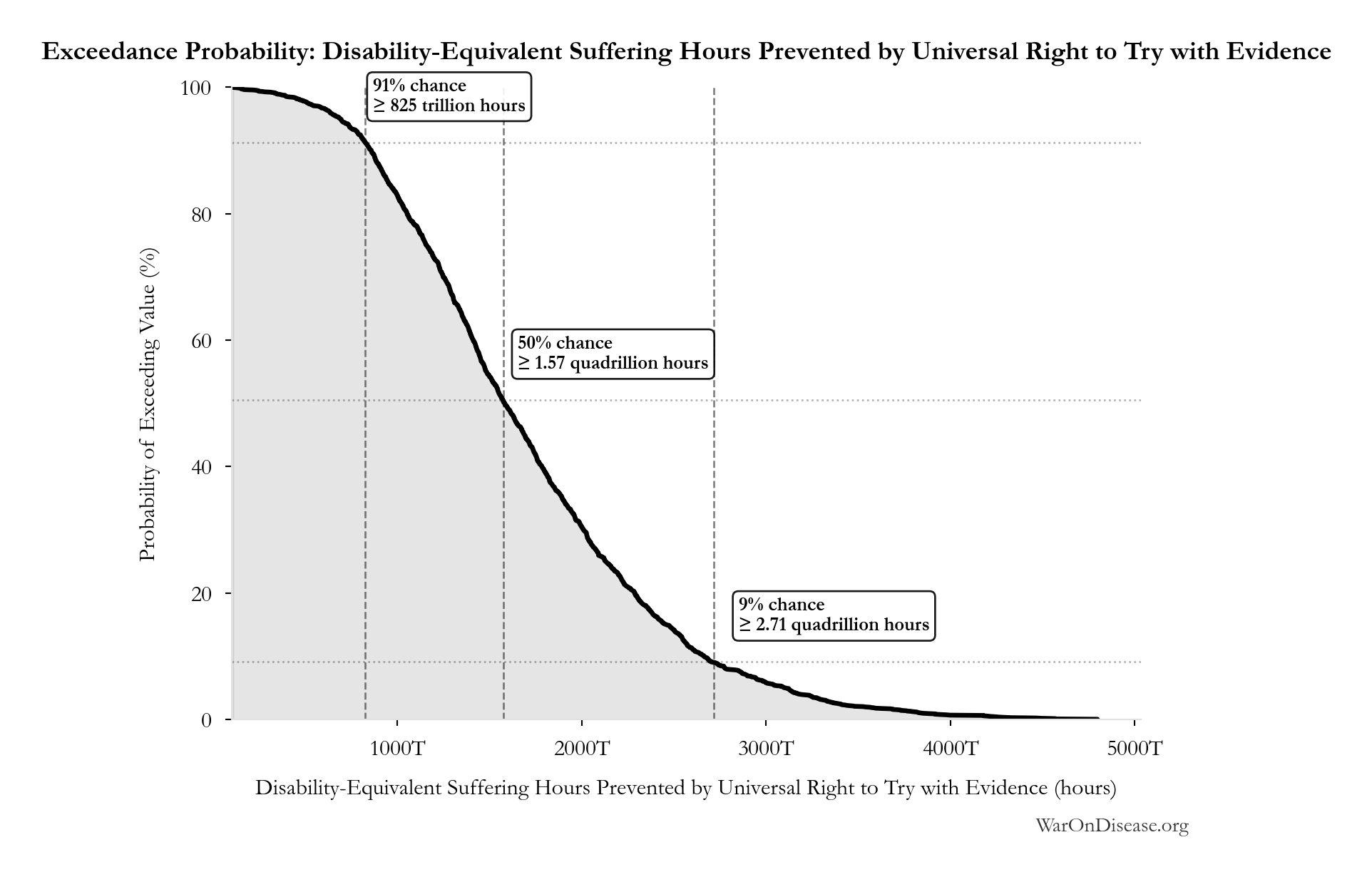
This exceedance probability chart shows the likelihood that Disability-Equivalent Suffering Hours Prevented by Universal Right to Try with Evidence will exceed any given threshold. Higher curves indicate more favorable outcomes with greater certainty.
Average Treatment Acceleration from Universal Right to Try with Evidence: 181 years
Note📊 Details
Average years earlier the first effective treatment arrives across the global therapeutic frontier after all 50 states adopt Universal Right to Try with Evidence. Uses the same schedule-shift structure as the 1% Treaty impact model: the status quo discovery timeline multiplied by one minus the inverse treatment-discovery multiplier.
Inputs:
- Status Quo Average Years to First Treatment 🔢: 222 years
- Universal Right to Try with Evidence Treatment Discovery Multiplier: 5.48x (95% CI: 1.1x - 15x)
\[ \begin{gathered} T_{accel,RTT} \\ = T_{first,SQ} \times \left(1 - \frac{1}{k_{RTT}}\right) \\ = 222 \times \left(1 - \frac{1}{5.48}\right) \\ = 181 \end{gathered} \] where: \[ \begin{gathered} T_{first,SQ} \\ = T_{queue,SQ} \times 0.5 \\ = 443 \times 0.5 \\ = 222 \end{gathered} \] where: \[ \begin{gathered} T_{queue,SQ} \\ = \frac{N_{untreated}}{Treatments_{new,ann}} \\ = \frac{6{,}650}{15} \\ = 443 \end{gathered} \] where: \[ \begin{gathered} N_{untreated} \\ = N_{rare} \times 0.95 \\ = 7{,}000 \times 0.95 \\ = 6{,}650 \end{gathered} \] ? Low confidence
Sensitivity Analysis
Sensitivity Indices for Average Treatment Acceleration from Universal Right to Try with Evidence
Regression-based sensitivity showing which inputs explain the most variance in the output.
| Input Parameter | Sensitivity Coefficient | Interpretation |
|---|---|---|
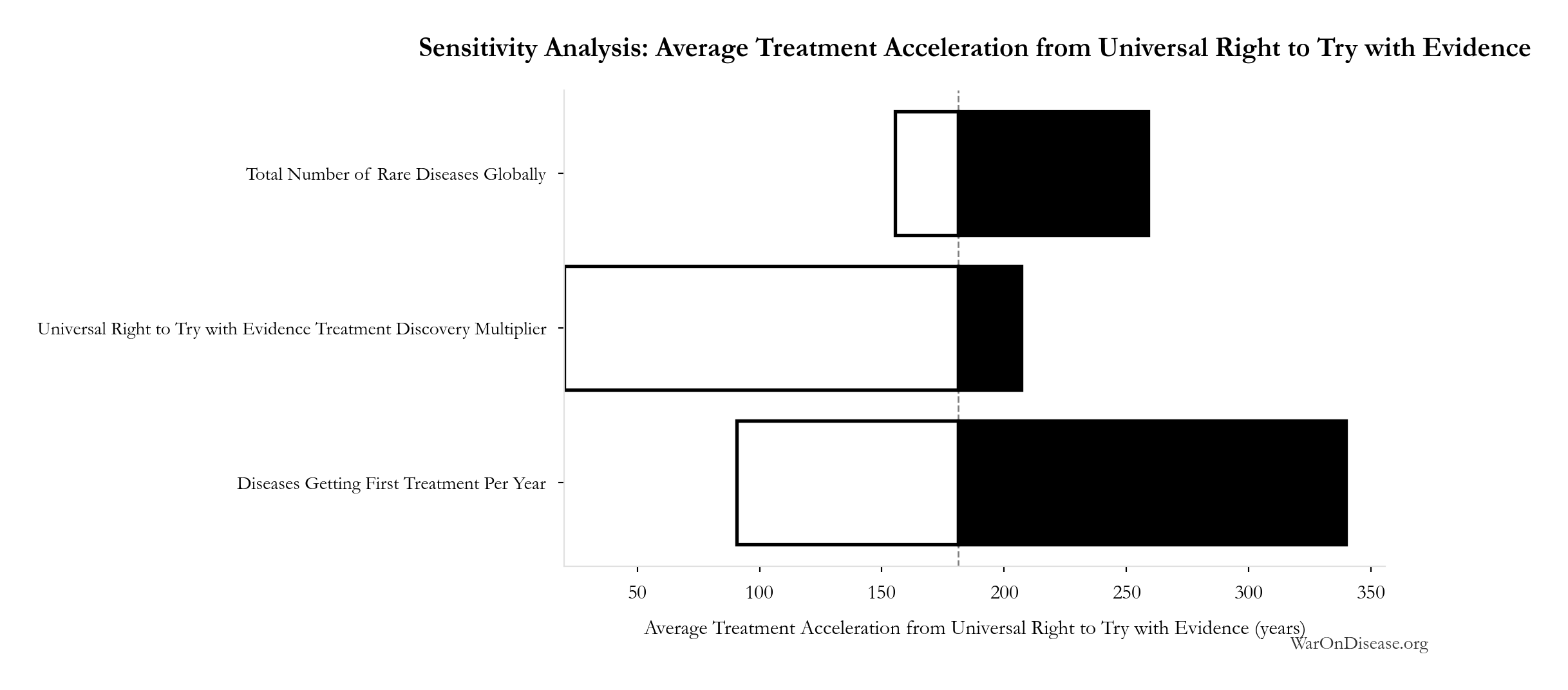
| Status Quo Average Years to First Treatment (years) | 0.8444 | Strong driver |
| Universal Right to Try with Evidence Treatment Discovery Multiplier (x) | 0.3959 | Moderate driver |
Interpretation: Standardized coefficients show the change in output (in SD units) per 1 SD change in input. Values near ±1 indicate strong influence; values exceeding ±1 may occur with correlated inputs.
Monte Carlo Distribution
Simulation Results Summary: Average Treatment Acceleration from Universal Right to Try with Evidence
| Statistic | Value |
|---|---|
| Baseline (deterministic) | 181 |
| Mean (expected value) | 187 |
| Median (50th percentile) | 176 |
| Standard Deviation | 77.8 |
| 90% Range (5th-95th percentile) | [79.1, 332] |
The histogram shows the distribution of Average Treatment Acceleration from Universal Right to Try with Evidence across 10,000 Monte Carlo simulations. The CDF (right) shows the probability of the outcome exceeding any given value, which is useful for risk assessment.
Exceedance Probability
This exceedance probability chart shows the likelihood that Average Treatment Acceleration from Universal Right to Try with Evidence will exceed any given threshold. Higher curves indicate more favorable outcomes with greater certainty.
Universal Right to Try with Evidence Cost-Effectiveness vs GiveWell Range Midpoint: 636.2kx
Note📊 Details
Conditional philanthropic cost-effectiveness of adopting Universal Right to Try with Evidence in all 50 states relative to the midpoint of GiveWell’s cited modeled cost-per-life-saved range. The cost scopes differ: the Right to Try numerator excludes patient and payer spending on treatment delivery, trial-site services, and permitted study costs, while the GiveWell figure includes full program costs. This comparison is valid only if full adoption and mature implementation produce the modeled treatment schedule shift.
Inputs:
- GiveWell Midpoint of Modeled Cost per Life Saved Range 📊: $4,500
- Universal Right to Try with Evidence Philanthropic Cost per Life Saved 🔢: $0.00707
\[ \begin{gathered} k_{RTT,GiveWell} \\ = \frac{Cost_{GW,avg}}{Cost_{RTT,life}} \\ = \frac{\$4.5K}{\$0.00707} \\ = 636{,}000 \end{gathered} \] where: \[ \begin{gathered} Cost_{RTT,life} \\ = \frac{C_{RTT}}{Lives_{RTT}} \\ = \frac{\$65M}{9.19B} \\ = \$0.00707 \end{gathered} \] where: \[ \begin{gathered} Lives_{RTT} \\ = Deaths_{disease,daily} \times Pct_{avoid,death} \times T_{accel,RTT} \times 365 \\ = 150{,}000 \times 92.6\% \times 181 \times 365 \\ = 9.19B \end{gathered} \] where: \[ \begin{gathered} T_{accel,RTT} \\ = T_{first,SQ} \times \left(1 - \frac{1}{k_{RTT}}\right) \\ = 222 \times \left(1 - \frac{1}{5.48}\right) \\ = 181 \end{gathered} \] where: \[ \begin{gathered} T_{first,SQ} \\ = T_{queue,SQ} \times 0.5 \\ = 443 \times 0.5 \\ = 222 \end{gathered} \] where: \[ \begin{gathered} T_{queue,SQ} \\ = \frac{N_{untreated}}{Treatments_{new,ann}} \\ = \frac{6{,}650}{15} \\ = 443 \end{gathered} \] where: \[ \begin{gathered} N_{untreated} \\ = N_{rare} \times 0.95 \\ = 7{,}000 \times 0.95 \\ = 6{,}650 \end{gathered} \] ? Low confidence
Sensitivity Analysis
Sensitivity Indices for Universal Right to Try with Evidence Cost-Effectiveness vs GiveWell Range Midpoint
Regression-based sensitivity showing which inputs explain the most variance in the output.
| Input Parameter | Sensitivity Coefficient | Interpretation |
|---|---|---|
| Universal Right to Try with Evidence Philanthropic Cost per Life Saved (USD/life) | -0.5292 | Strong driver |
Interpretation: Standardized coefficients show the change in output (in SD units) per 1 SD change in input. Values near ±1 indicate strong influence; values exceeding ±1 may occur with correlated inputs.
Monte Carlo Distribution
Simulation Results Summary: Universal Right to Try with Evidence Cost-Effectiveness vs GiveWell Range Midpoint
| Statistic | Value |
|---|---|
| Baseline (deterministic) | 636.2kx |
| Mean (expected value) | 881.6kx |
| Median (50th percentile) | 717.9kx |
| Standard Deviation | 629.4kx |
| 90% Range (5th-95th percentile) | [190.7kx, 2.1Mx] |
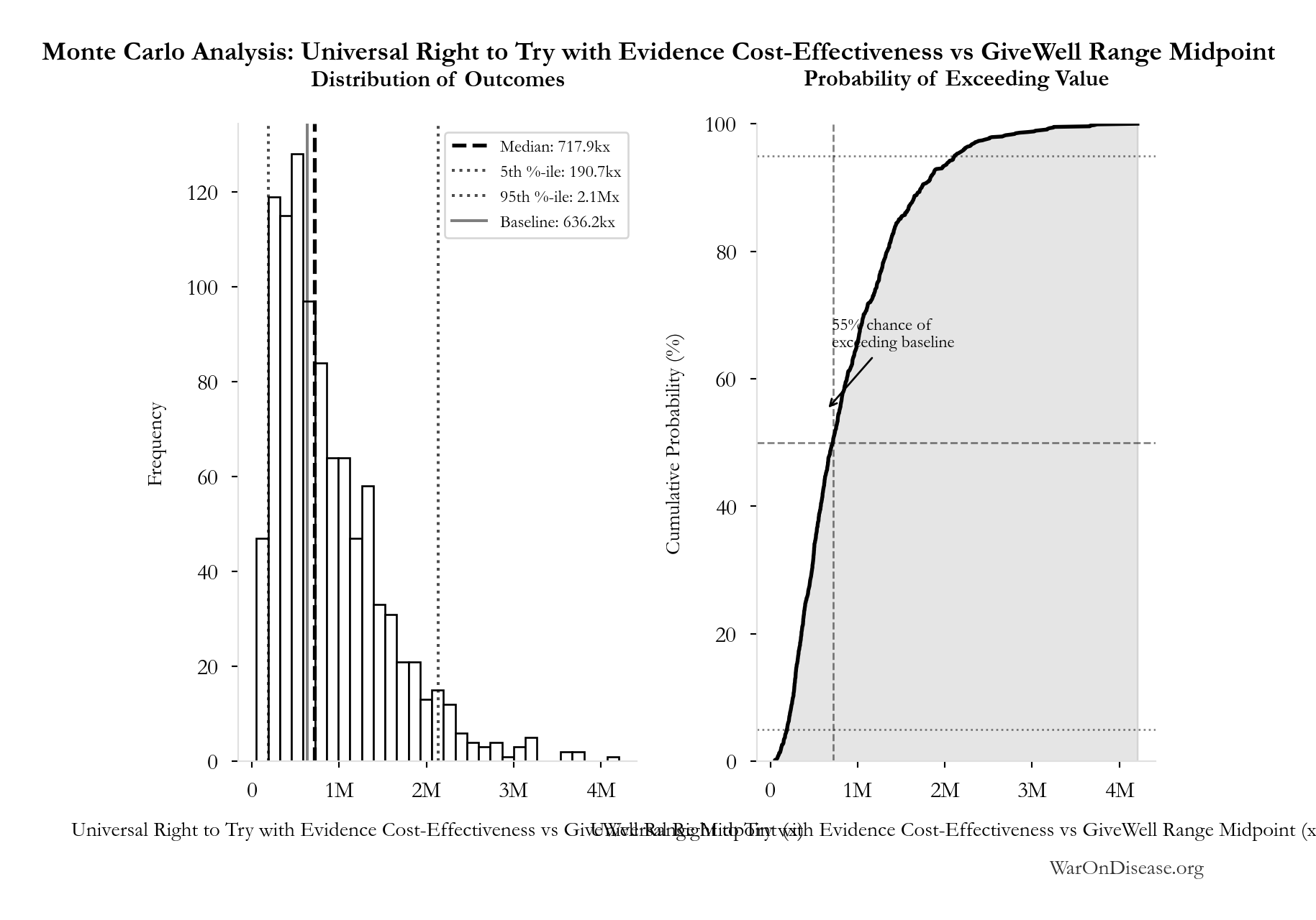
The histogram shows the distribution of Universal Right to Try with Evidence Cost-Effectiveness vs GiveWell Range Midpoint across 10,000 Monte Carlo simulations. The CDF (right) shows the probability of the outcome exceeding any given value, which is useful for risk assessment.
Exceedance Probability
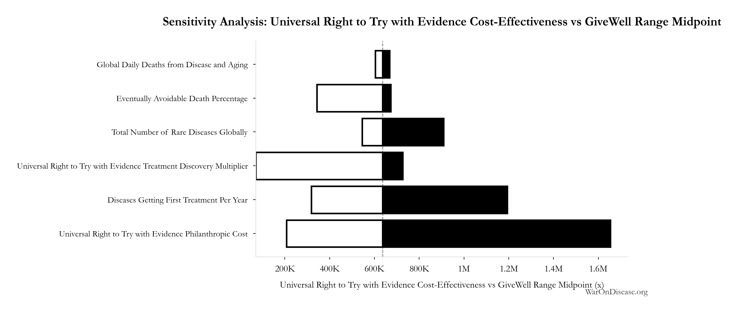
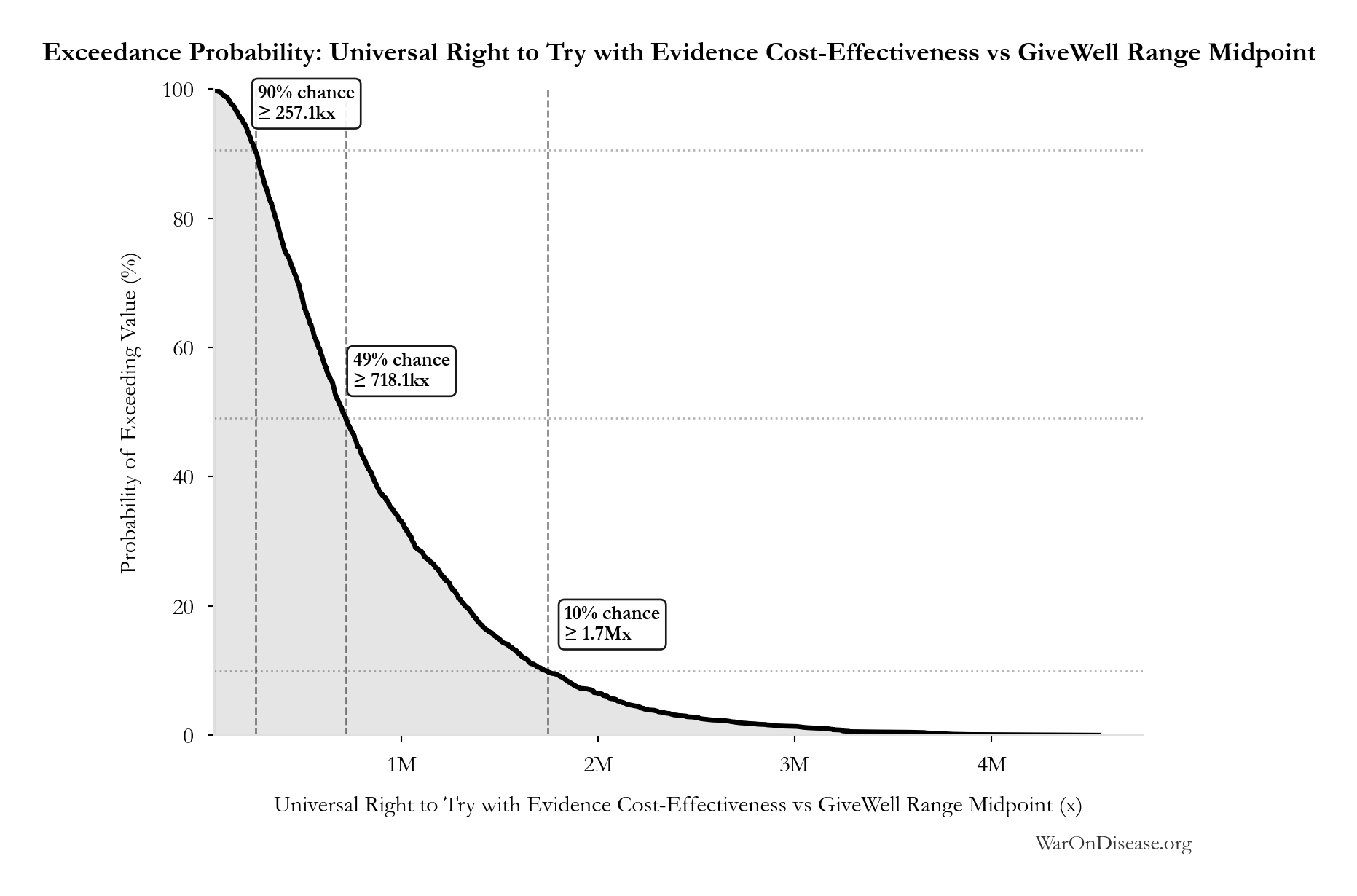
This exceedance probability chart shows the likelihood that Universal Right to Try with Evidence Cost-Effectiveness vs GiveWell Range Midpoint will exceed any given threshold. Higher curves indicate more favorable outcomes with greater certainty.
Status Quo Average Years to First Treatment: 222 years
Note📊 Details
Average years until first treatment discovered for a typical disease under current system. At current discovery rates, the average disease waits half the total exploration time (~443/2 = ~222 years).
Inputs:
- Status Quo Therapeutic Space Exploration Time 🔢: 443 years
\[ \begin{gathered} T_{first,SQ} \\ = T_{queue,SQ} \times 0.5 \\ = 443 \times 0.5 \\ = 222 \end{gathered} \] where: \[ \begin{gathered} T_{queue,SQ} \\ = \frac{N_{untreated}}{Treatments_{new,ann}} \\ = \frac{6{,}650}{15} \\ = 443 \end{gathered} \] where: \[ \begin{gathered} N_{untreated} \\ = N_{rare} \times 0.95 \\ = 7{,}000 \times 0.95 \\ = 6{,}650 \end{gathered} \] Methodology:4
? Low confidence
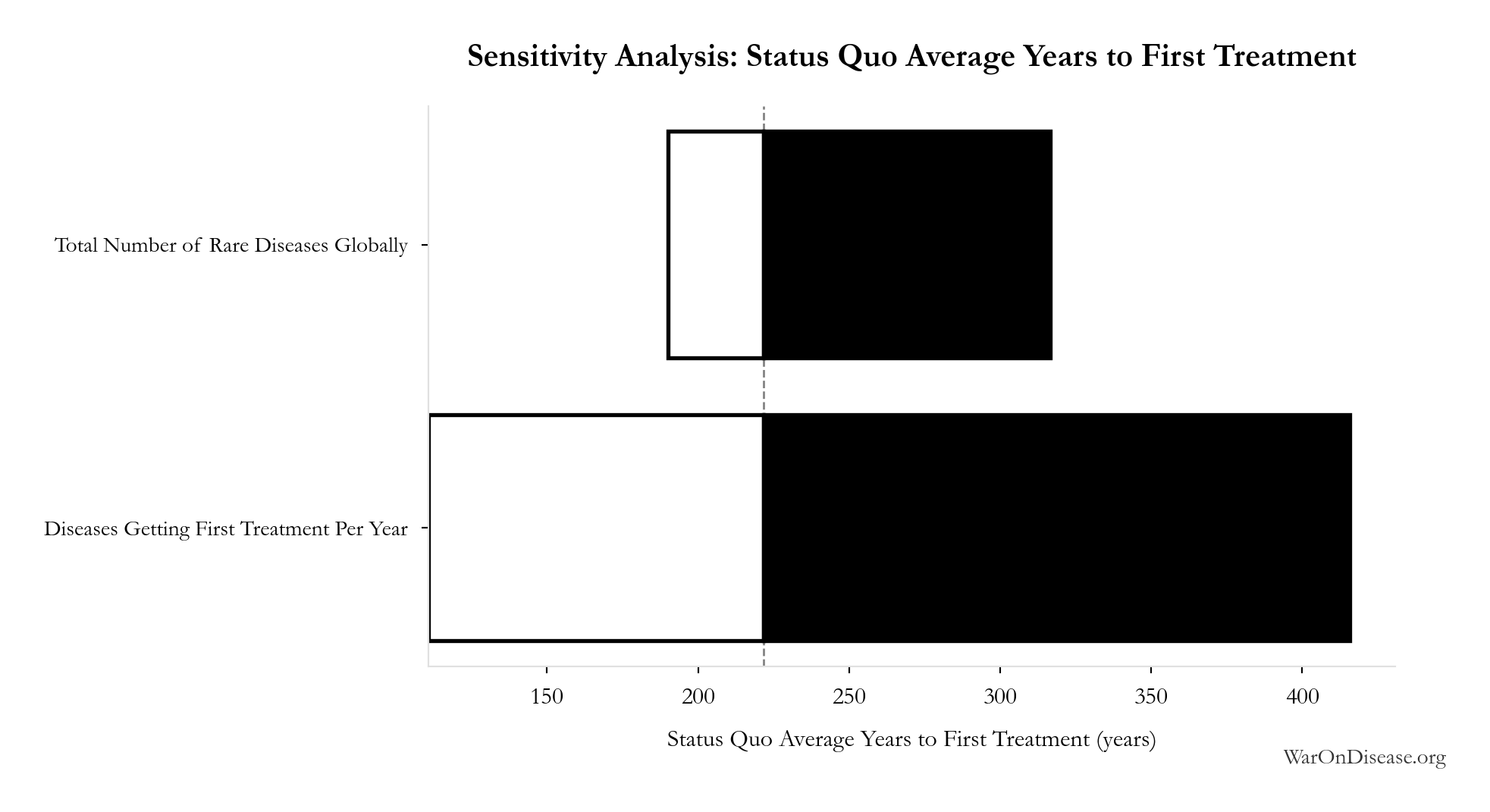
Sensitivity Analysis
Sensitivity Indices for Status Quo Average Years to First Treatment
Regression-based sensitivity showing which inputs explain the most variance in the output.
| Input Parameter | Sensitivity Coefficient | Interpretation |
|---|---|---|
| Status Quo Therapeutic Space Exploration Time (years) | 1.0000 | Strong driver |
Interpretation: Standardized coefficients show the change in output (in SD units) per 1 SD change in input. Values near ±1 indicate strong influence; values exceeding ±1 may occur with correlated inputs.
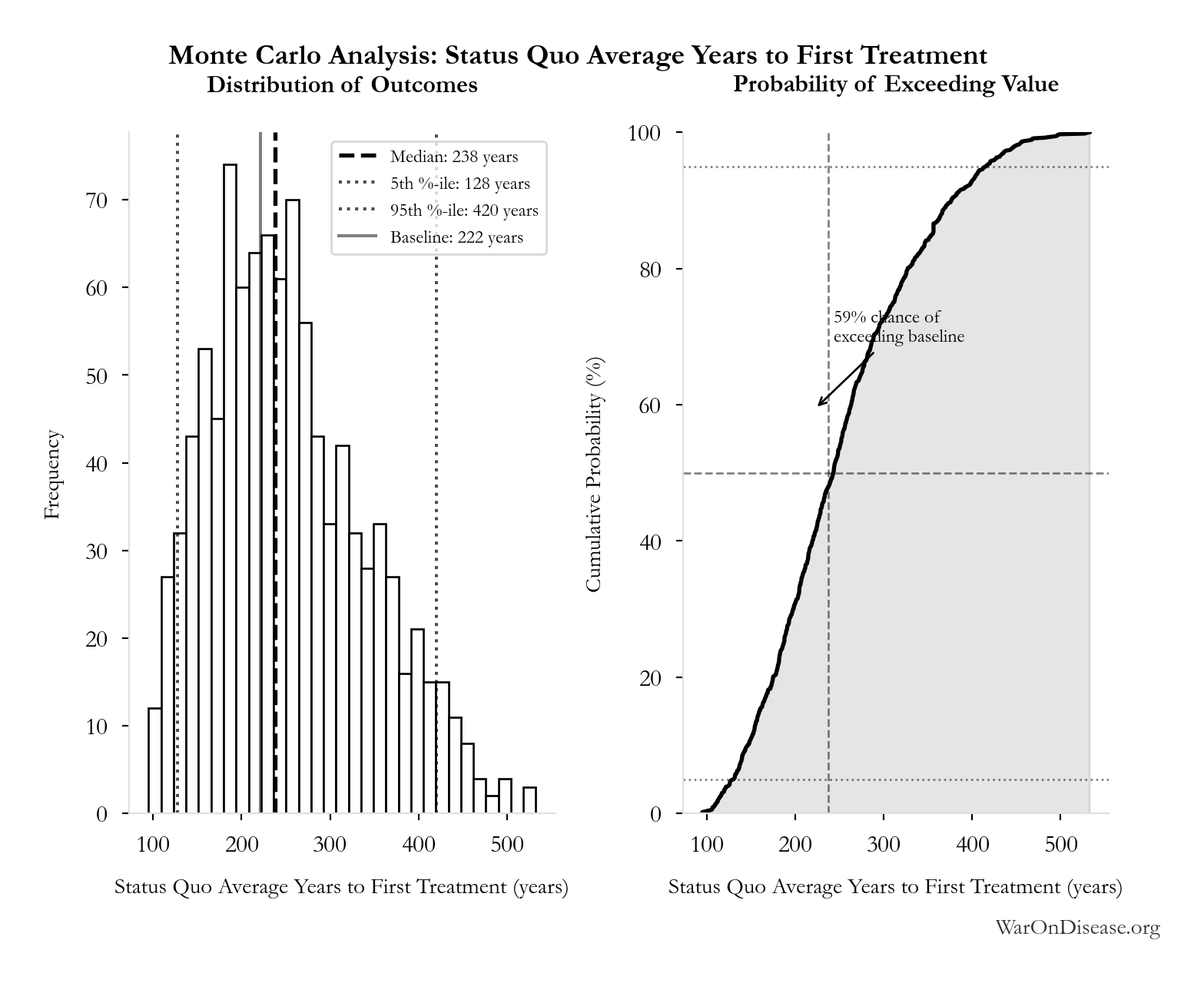
Monte Carlo Distribution
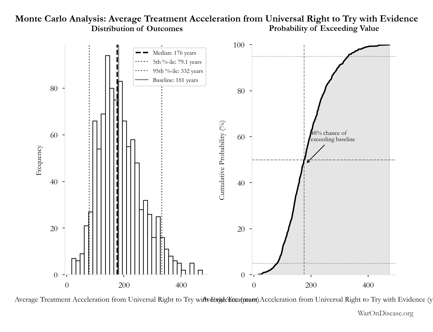
Simulation Results Summary: Status Quo Average Years to First Treatment
| Statistic | Value |
|---|---|
| Baseline (deterministic) | 222 |
| Mean (expected value) | 251 |
| Median (50th percentile) | 238 |
| Standard Deviation | 88.8 |
| 90% Range (5th-95th percentile) | [128, 420] |
The histogram shows the distribution of Status Quo Average Years to First Treatment across 10,000 Monte Carlo simulations. The CDF (right) shows the probability of the outcome exceeding any given value, which is useful for risk assessment.
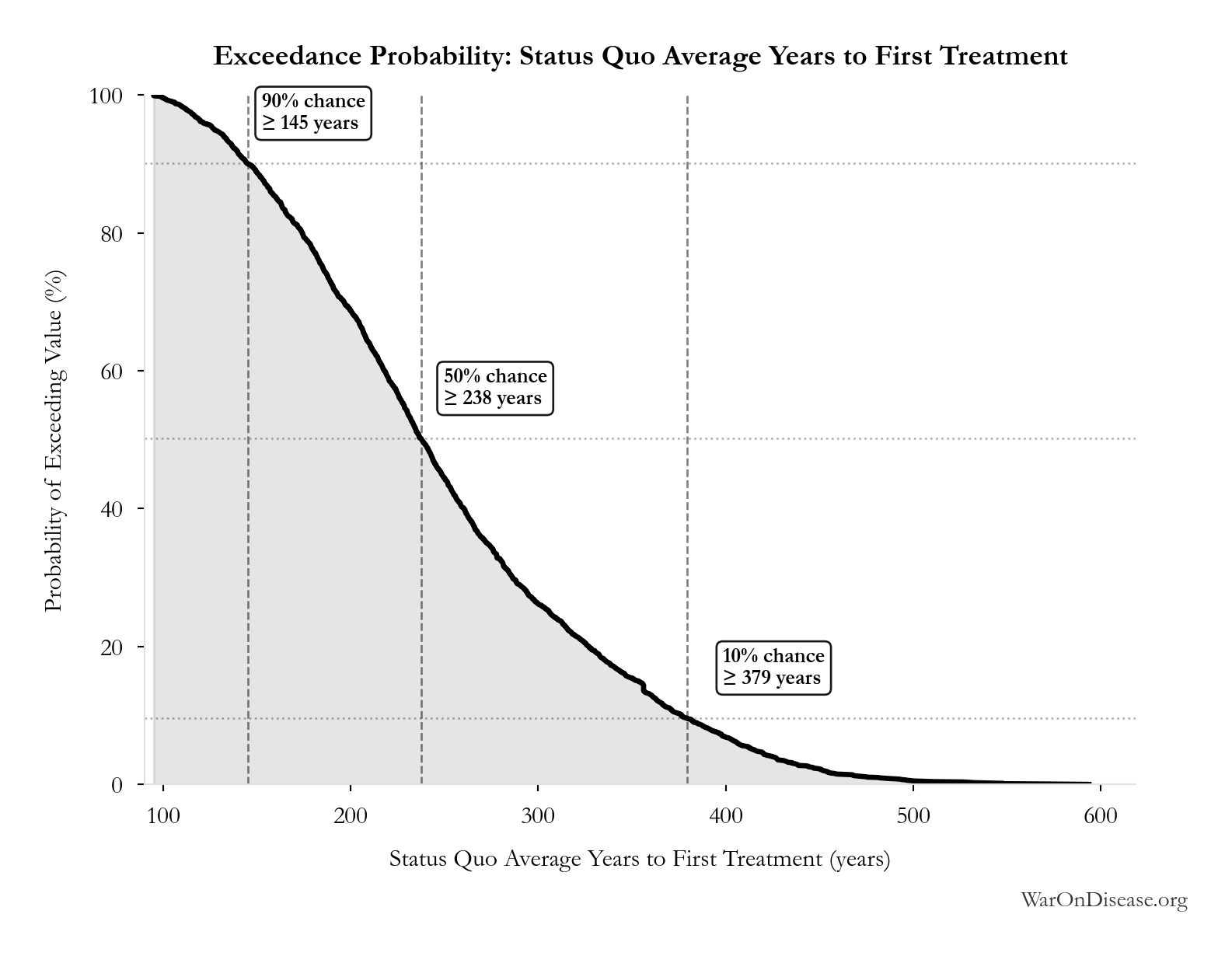
Exceedance Probability
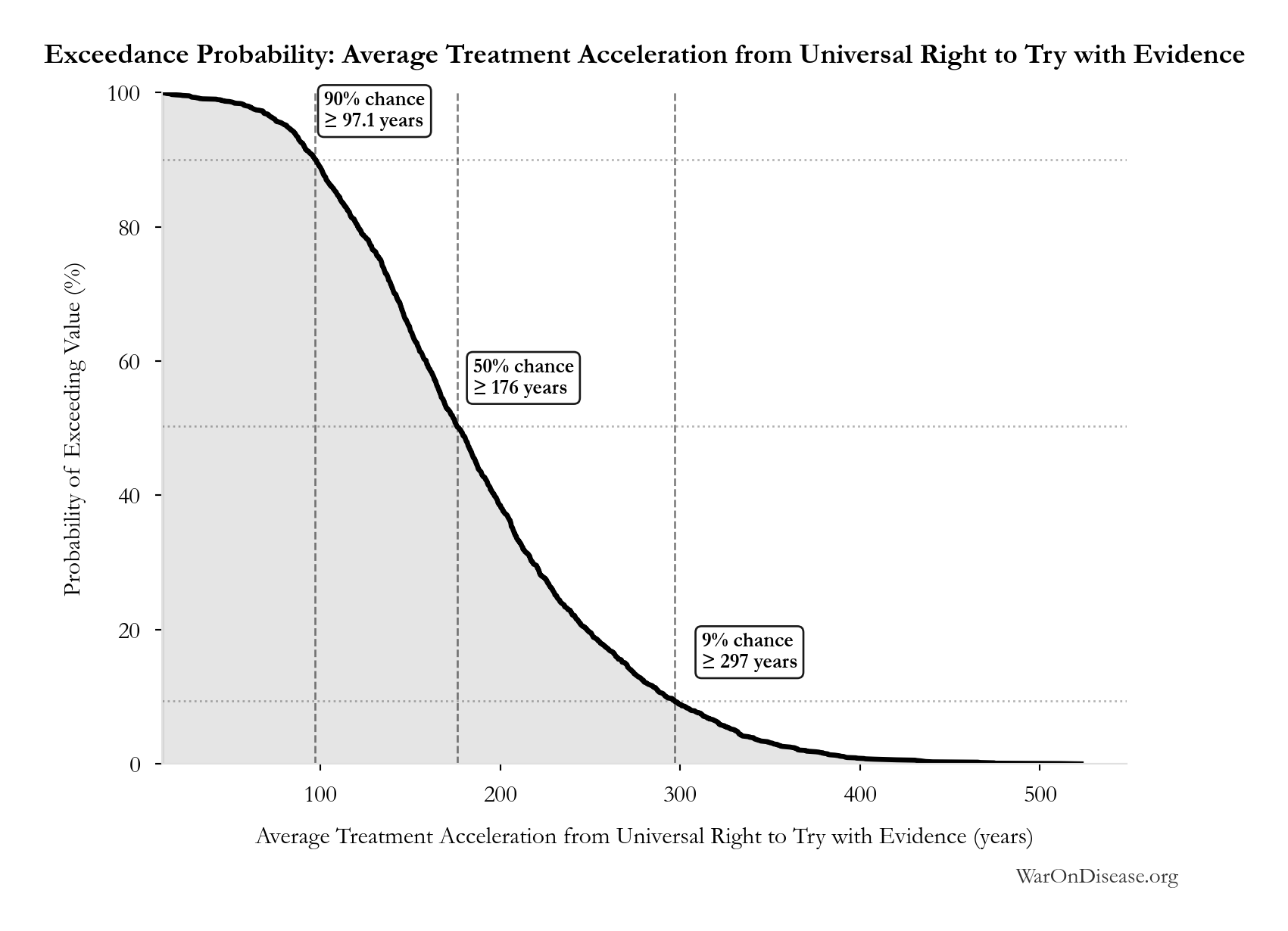
This exceedance probability chart shows the likelihood that Status Quo Average Years to First Treatment will exceed any given threshold. Higher curves indicate more favorable outcomes with greater certainty.
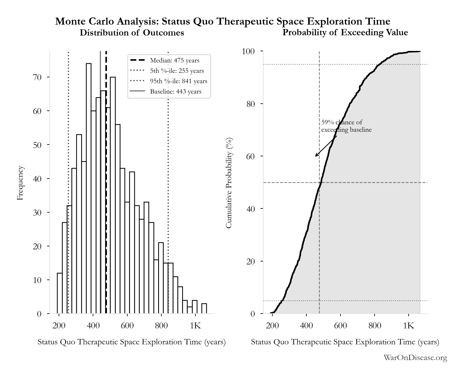
Status Quo Therapeutic Space Exploration Time: 443 years
Note📊 Details
Years to explore the entire therapeutic search space under current system. At current discovery rate of ~15 diseases/year getting first treatments, finding treatments for all ~6,650 untreated diseases would take ~443 years.
Inputs:
- Diseases Without Effective Treatment 🔢: 6,650 diseases
- Diseases Getting First Treatment Per Year 📊: 15 diseases/year (95% CI: 8 diseases/year - 30 diseases/year)
\[ \begin{gathered} T_{queue,SQ} \\ = \frac{N_{untreated}}{Treatments_{new,ann}} \\ = \frac{6{,}650}{15} \\ = 443 \end{gathered} \] where: \[ \begin{gathered} N_{untreated} \\ = N_{rare} \times 0.95 \\ = 7{,}000 \times 0.95 \\ = 6{,}650 \end{gathered} \] Methodology:4
? Low confidence
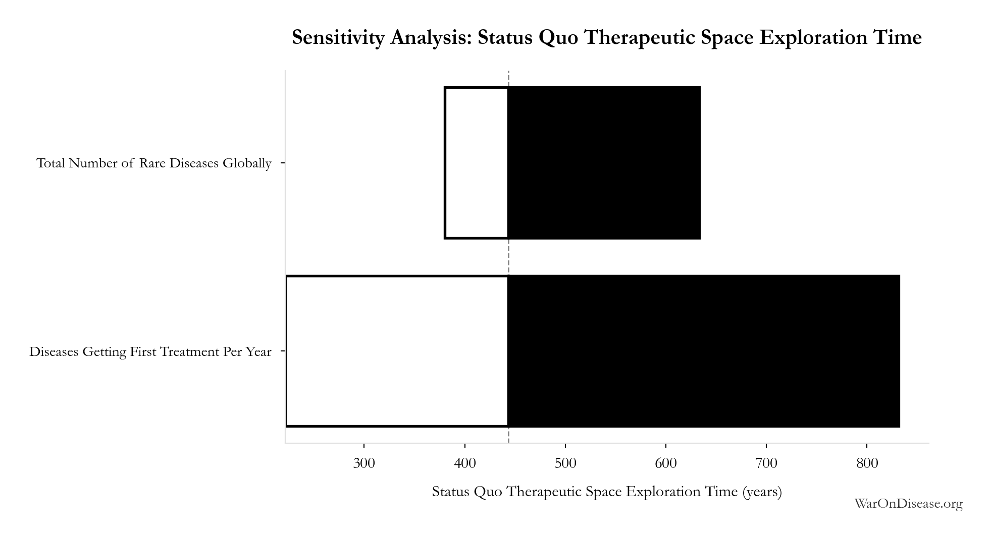
Sensitivity Analysis
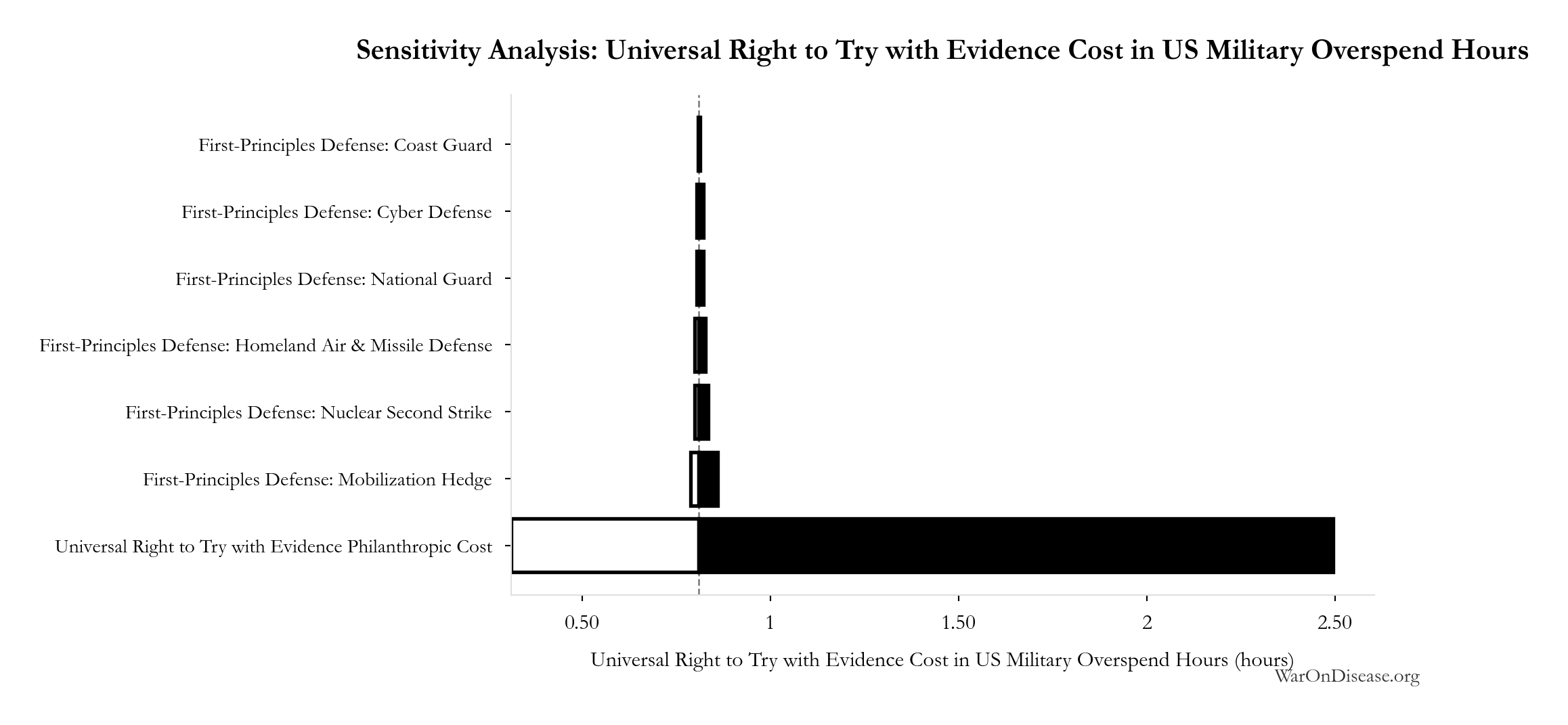
Sensitivity Indices for Status Quo Therapeutic Space Exploration Time
Regression-based sensitivity showing which inputs explain the most variance in the output.
| Input Parameter | Sensitivity Coefficient | Interpretation |
|---|---|---|
| Diseases Getting First Treatment Per Year (diseases/year) | -0.8696 | Strong driver |
| Diseases Without Effective Treatment (diseases) | 0.3427 | Moderate driver |
Interpretation: Standardized coefficients show the change in output (in SD units) per 1 SD change in input. Values near ±1 indicate strong influence; values exceeding ±1 may occur with correlated inputs.
Monte Carlo Distribution
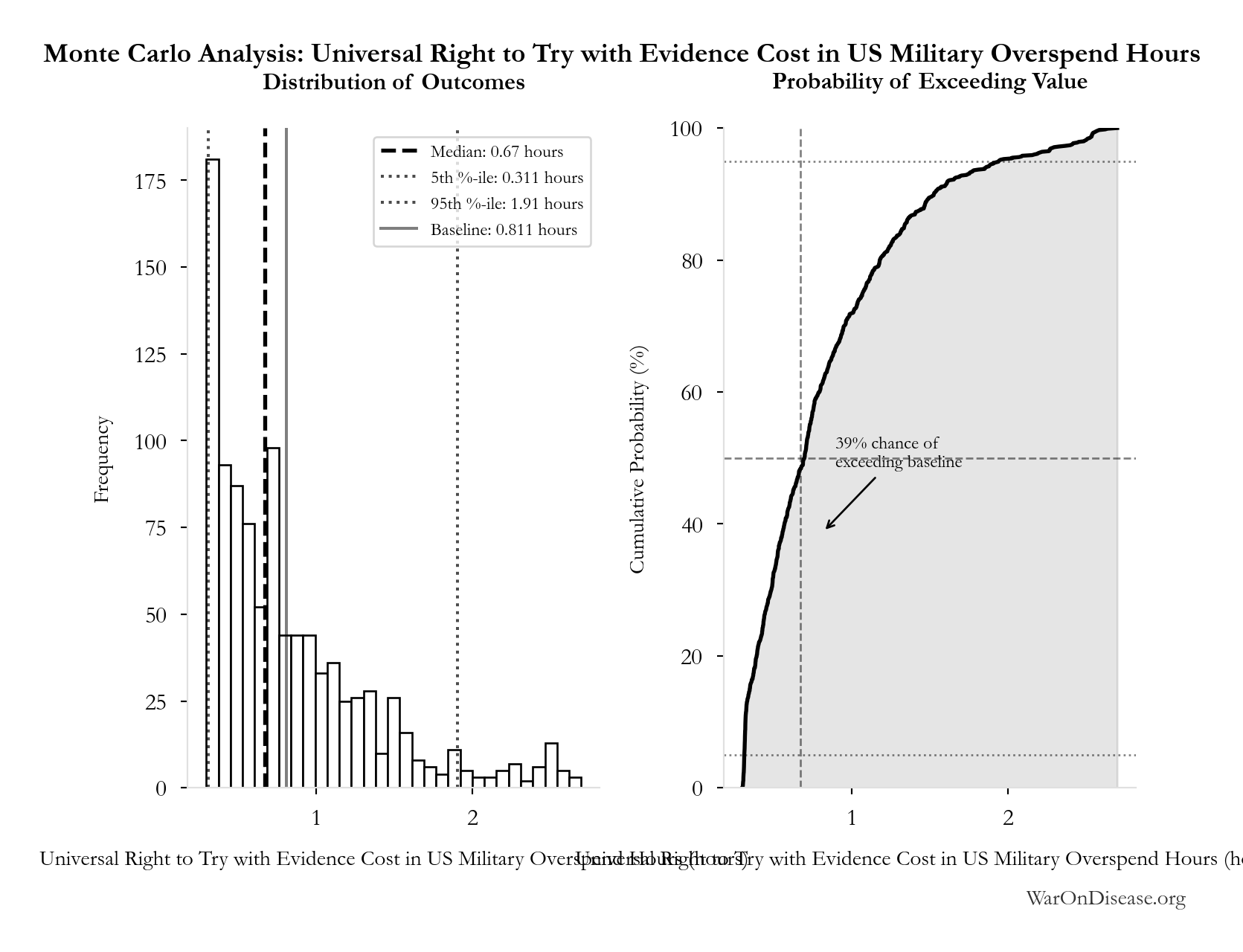
Simulation Results Summary: Status Quo Therapeutic Space Exploration Time
| Statistic | Value |
|---|---|
| Baseline (deterministic) | 443 |
| Mean (expected value) | 502 |
| Median (50th percentile) | 475 |
| Standard Deviation | 178 |
| 90% Range (5th-95th percentile) | [255, 841] |
The histogram shows the distribution of Status Quo Therapeutic Space Exploration Time across 10,000 Monte Carlo simulations. The CDF (right) shows the probability of the outcome exceeding any given value, which is useful for risk assessment.
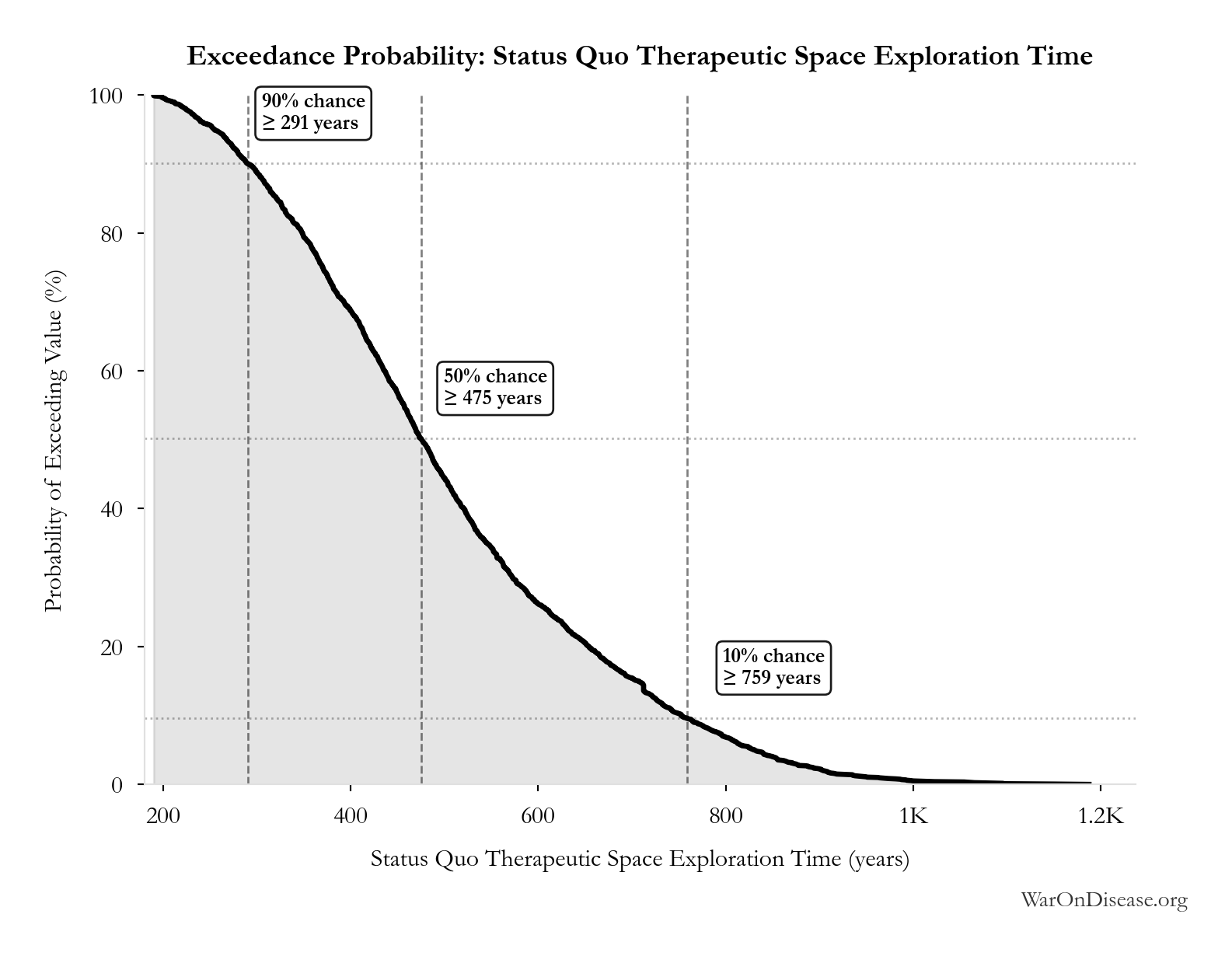
Exceedance Probability
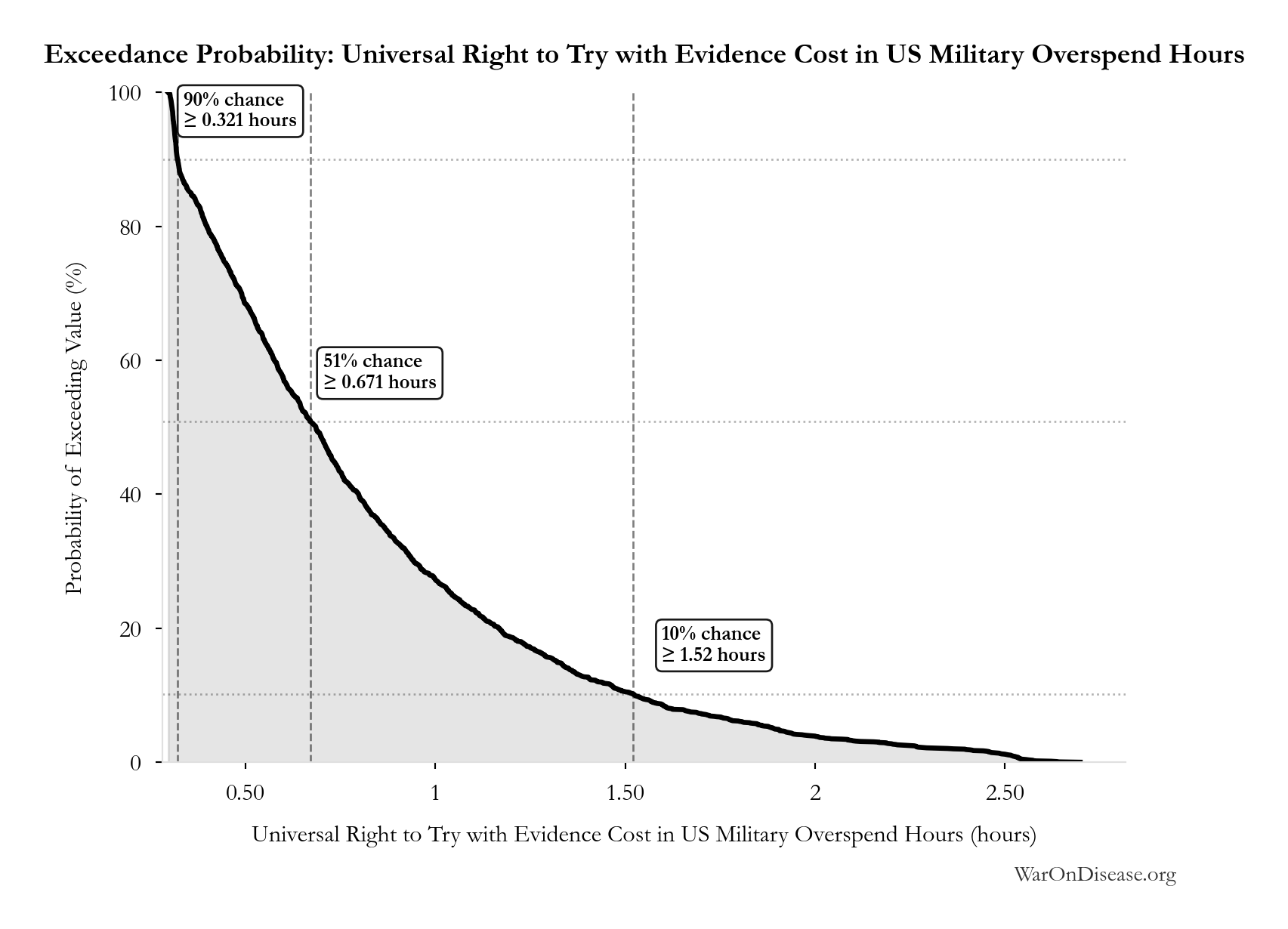
This exceedance probability chart shows the likelihood that Status Quo Therapeutic Space Exploration Time will exceed any given threshold. Higher curves indicate more favorable outcomes with greater certainty.
External Data Sources
Parameters sourced from peer-reviewed publications, institutional databases, and authoritative reports.
Pragmatic Trial Cost per Patient: $929
Note📊 Details
Embedded pragmatic trial cost per patient. Uses ADAPTABLE trial ($929) as DELIBERATELY CONSERVATIVE central estimate. Ramsberg & Platt (2018) reviewed 108 embedded pragmatic trials; 64 with cost data had median of only $97/patient - this estimate may overstate costs by 10x. Confidence interval spans meta-analysis median to complex chronic disease trials.
Source:1
Uncertainty Range
Technical: 95% CI: [$97, $3,000] • Distribution: Lognormal
What this means: This estimate is highly uncertain. The true value likely falls between $97 and $3,000 (±156%). This represents a very wide range that our Monte Carlo simulations account for when calculating overall uncertainty in the results.
The lognormal distribution means values can’t go negative and have a longer tail toward higher values (common for costs and populations).
Input Distribution
This chart shows the assumed probability distribution for this parameter. The shaded region represents the 95% confidence interval where we expect the true value to fall.
~ Medium confidence
GiveWell Midpoint of Modeled Cost per Life Saved Range: $4,500
Note📊 Details
Midpoint of GiveWell’s cited $3,500 to $5,500 modeled cost-per-life-saved range across top charities
Source:5
Uncertainty Range
Technical: Distribution: Fixed
✓ High confidence
Global Annual DALY Burden: 2.88 billion DALYs/year
Note📊 Details
Global annual DALY burden from all diseases and injuries (WHO/IHME Global Burden of Disease 2021). Includes both YLL (years of life lost) and YLD (years lived with disability) from all causes.
Source:6
Uncertainty Range
Technical: Distribution: Normal (SE: 150 million DALYs/year)
Input Distribution
This chart shows the assumed probability distribution for this parameter. The shaded region represents the 95% confidence interval where we expect the true value to fall.
✓ High confidence • 📊 Peer-reviewed
Global Daily Deaths from Disease and Aging: 150 thousand deaths/day
Note📊 Details
Total global deaths per day from all disease and aging (WHO Global Burden of Disease 2024)
Source:7
Uncertainty Range
Technical: Distribution: Normal (SE: 7,500 deaths/day)
Input Distribution
This chart shows the assumed probability distribution for this parameter. The shaded region represents the 95% confidence interval where we expect the true value to fall.
✓ High confidence • 📊 Peer-reviewed
YLD Proportion of Total DALYs: 0.39 proportion
Note📊 Details
Proportion of global DALYs that are YLD (years lived with disability) vs YLL (years of life lost). From GBD 2021: 1.13B YLD out of 2.88B total DALYs = 39%.
Source:6
Uncertainty Range
Technical: Distribution: Normal (SE: 0.03 proportion)
Input Distribution
This chart shows the assumed probability distribution for this parameter. The shaded region represents the 95% confidence interval where we expect the true value to fall.
✓ High confidence • 📊 Peer-reviewed
Diseases Getting First Treatment Per Year: 15 diseases/year
Note📊 Details
Number of diseases that receive their FIRST effective treatment each year under current system. ~9 rare diseases/year (based on 40 years of ODA: 350 with treatment ÷ 40 years), plus ~5-10 common diseases. Note: FDA approves ~50 drugs/year, but most are for diseases that already have treatments.
Source:8
Uncertainty Range
Technical: 95% CI: [8 diseases/year, 30 diseases/year] • Distribution: Lognormal
What this means: This estimate is highly uncertain. The true value likely falls between 8 diseases/year and 30 diseases/year (±73%). This represents a very wide range that our Monte Carlo simulations account for when calculating overall uncertainty in the results.
The lognormal distribution means values can’t go negative and have a longer tail toward higher values (common for costs and populations).
Input Distribution
This chart shows the assumed probability distribution for this parameter. The shaded region represents the 95% confidence interval where we expect the true value to fall.
? Low confidence
Total Number of Rare Diseases Globally: 7,000 diseases
Note📊 Details
Total number of rare diseases globally
Source:9
Uncertainty Range
Technical: 95% CI: [6,000 diseases, 10,000 diseases] • Distribution: Normal
What this means: There’s significant uncertainty here. The true value likely falls between 6,000 diseases and 10,000 diseases (±29%). This represents a wide range that our Monte Carlo simulations account for when calculating overall uncertainty in the results.
The normal distribution means values cluster around the center with equal chances of being higher or lower.
Input Distribution
This chart shows the assumed probability distribution for this parameter. The shaded region represents the 95% confidence interval where we expect the true value to fall.
✓ High confidence
Phase 3 Cost per Patient: $41,000
Note📊 Details
Phase 3 cost per patient (median from FDA study)
Source:2
Uncertainty Range
Technical: 95% CI: [$20,000, $120,000] • Distribution: Lognormal
What this means: This estimate is highly uncertain. The true value likely falls between $20,000 and $120,000 (±122%). This represents a very wide range that our Monte Carlo simulations account for when calculating overall uncertainty in the results.
The lognormal distribution means values can’t go negative and have a longer tail toward higher values (common for costs and populations).
Input Distribution
This chart shows the assumed probability distribution for this parameter. The shaded region represents the 95% confidence interval where we expect the true value to fall.
✓ High confidence
Core Definitions
Fundamental parameters and constants used throughout the analysis.
Eventually Avoidable DALY Percentage: 92.6%
Note📊 Details
Percentage of DALYs that are eventually avoidable with sufficient biomedical research. Uses same methodology as EVENTUALLY_AVOIDABLE_DEATH_PCT. Most non-fatal chronic conditions (arthritis, depression, chronic pain) are also addressable through research, so the percentage is similar to deaths.
Uncertainty Range
Technical: 95% CI: [50%, 98%] • Distribution: Beta
What this means: There’s significant uncertainty here. The true value likely falls between 50% and 98% (±26%). This represents a wide range that our Monte Carlo simulations account for when calculating overall uncertainty in the results.
The beta distribution means values are bounded and can skew toward one end.
Input Distribution
This chart shows the assumed probability distribution for this parameter. The shaded region represents the 95% confidence interval where we expect the true value to fall.
Core definition
Eventually Avoidable Death Percentage: 92.6%
Note📊 Details
Percentage of deaths that are eventually avoidable with sufficient biomedical research and technological advancement. Central estimate ~92% based on ~7.9% fundamentally unavoidable (primarily accidents). Wide uncertainty reflects debate over: (1) aging as addressable vs. fundamental, (2) asymptotic difficulty of last diseases, (3) multifactorial disease complexity.
Uncertainty Range
Technical: 95% CI: [50%, 98%] • Distribution: Beta
What this means: There’s significant uncertainty here. The true value likely falls between 50% and 98% (±26%). This represents a wide range that our Monte Carlo simulations account for when calculating overall uncertainty in the results.
The beta distribution means values are bounded and can skew toward one end.
Input Distribution
This chart shows the assumed probability distribution for this parameter. The shaded region represents the 95% confidence interval where we expect the true value to fall.
Core definition
Universal Right to Try with Evidence Philanthropic Cost: $65 million
Note📊 Details
Total philanthropic cost of adopting Universal Right to Try with Evidence in all 50 states: a central $15 million campaign estimate covering legislation or amendment in all 50 states plus $50 million for the shared registry’s first ten years. The model bill requires participating centers to fund continued registry operation after year ten. This philanthropic numerator excludes patient or payer spending on treatment delivery, trial-site services, and permitted study costs. The wide interval represents campaign and infrastructure cost uncertainty without separate scenario parameters.
Uncertainty Range
Technical: 95% CI: [$25 million, $200 million] • Distribution: Lognormal
What this means: This estimate is highly uncertain. The true value likely falls between $25 million and $200 million (±135%). This represents a very wide range that our Monte Carlo simulations account for when calculating overall uncertainty in the results.
The lognormal distribution means values can’t go negative and have a longer tail toward higher values (common for costs and populations).
Input Distribution
This chart shows the assumed probability distribution for this parameter. The shaded region represents the 95% confidence interval where we expect the true value to fall.
Core definition
Universal Right to Try with Evidence Treatment Discovery Multiplier: 5.48x
Note📊 Details
Conditional multiplier on the worldwide first-treatment discovery rate after all 50 states adopt and a mature pooled pragmatic-trial system operates under applicable federal authorization. The 5.48x central calibration reproduces the prior model’s 82.2 versus 15 first treatments per year; it is an assumption, not an observed effect estimate. This single input incorporates patient or payer funding of treatment delivery, trial-site services, and permitted study costs, newly viable post-Phase-1 treatment-condition pairs, evaluable protocol quality, candidate supply, and scientific success. Its range describes productivity of an operating system, not the separate probability that advocacy achieves full adoption and implementation.
Uncertainty Range
Technical: 95% CI: [1.1x, 15x] • Distribution: Lognormal
What this means: This estimate is highly uncertain. The true value likely falls between 1.1x and 15x (±127%). This represents a very wide range that our Monte Carlo simulations account for when calculating overall uncertainty in the results.
The lognormal distribution means values can’t go negative and have a longer tail toward higher values (common for costs and populations).
Input Distribution
This chart shows the assumed probability distribution for this parameter. The shaded region represents the 95% confidence interval where we expect the true value to fall.
Core definition
1.
NIH Common Fund. NIH pragmatic trials: Minimal funding despite 30x cost advantage. NIH Common Fund: HCS Research Collaboratory https://commonfund.nih.gov/hcscollaboratory (2025)
The NIH Pragmatic Trials Collaboratory funds trials at $500K for planning phase, $1M/year for implementation-a tiny fraction of NIH’s budget. The ADAPTABLE trial cost $14 million for 15,076 patients (= $929/patient) versus $420 million for a similar traditional RCT (30x cheaper), yet pragmatic trials remain severely underfunded. PCORnet infrastructure enables real-world trials embedded in healthcare systems, but receives minimal support compared to basic research funding. Additional sources: https://commonfund.nih.gov/hcscollaboratory | https://pcornet.org/wp-content/uploads/2025/08/ADAPTABLE_Lay_Summary_21JUL2025.pdf | https://www.ncbi.nlm.nih.gov/pmc/articles/PMC5604499/
.2.
FDA Study via NCBI. Trial costs, FDA study. FDA Study via NCBI https://www.ncbi.nlm.nih.gov/pmc/articles/PMC6248200/
Overall, the 138 clinical trials had an estimated median (IQR) cost of $19.0 million ($12.2 million-$33.1 million)... The clinical trials cost a median (IQR) of $41,117 ($31,802-$82,362) per patient. Additional sources: https://www.ncbi.nlm.nih.gov/pmc/articles/PMC6248200/
.3.
Orphanet Journal of Rare Diseases (2024). Rare disease treatment gap. Orphanet Journal of Rare Diseases (2024) https://ojrd.biomedcentral.com/articles/10.1186/s13023-024-03398-1 (2024)
Most patients wait 5 to 10 years to get an accurate diagnosis - and only about 5% of rare diseases have an FDA-approved treatment. Over the 40 years of the ODA, 6,340 orphan drug designations were granted, representing drug development for 1,079 rare diseases out of 7,000-10,000 known rare conditions.
4.
Composite estimate based on Orphanet. Average time to cure under current system.
Queue-based calculation: 7,000 diseases without effective treatment ÷ 15 diseases getting first treatment per year = 467 years for the average disease to receive a cure under the status quo system. This is consistent with the fact that only 5% of rare diseases have treatments after 40+ years of the Orphan Drug Act. Well-funded diseases may take 30-50 years; underfunded diseases 100-500+ years; and neglected diseases effectively never within human planning horizons.
5.
GiveWell. GiveWell cost per life saved for top charities (2024). GiveWell: Top Charities https://www.givewell.org/charities/top-charities
General range: $3,000-$5,500 per life saved (GiveWell top charities) Helen Keller International (Vitamin A): $3,500 average (2022-2024); varies $1,000-$8,500 by country Against Malaria Foundation: $5,500 per life saved New Incentives (vaccination incentives): $4,500 per life saved Malaria Consortium (seasonal malaria chemoprevention): $3,500 per life saved VAS program details: $2 to provide vitamin A supplements to child for one year Note: Figures accurate for 2024. Helen Keller VAS program has wide country variation ($1K-$8.5K) but $3,500 is accurate average. Among most cost-effective interventions globally Additional sources: https://www.givewell.org/charities/top-charities | https://www.givewell.org/charities/helen-keller-international | https://ourworldindata.org/cost-effectiveness
.6.
Institute for Health Metrics and Evaluation (IHME). IHME global burden of disease 2021 (2.88B DALYs, 1.13B YLD). Institute for Health Metrics and Evaluation (IHME) https://vizhub.healthdata.org/gbd-results/ (2024)
In 2021, global DALYs totaled approximately 2.88 billion, comprising 1.75 billion Years of Life Lost (YLL) and 1.13 billion Years Lived with Disability (YLD). This represents a 13% increase from 2019 (2.55B DALYs), largely attributable to COVID-19 deaths and aging populations. YLD accounts for approximately 39% of total DALYs, reflecting the substantial burden of non-fatal chronic conditions. Additional sources: https://vizhub.healthdata.org/gbd-results/ | https://www.thelancet.com/journals/lancet/article/PIIS0140-6736(24)00757-8/fulltext | https://www.healthdata.org/research-analysis/about-gbd
.7.
World Health Organization. WHO global health estimates 2024. World Health Organization https://www.who.int/data/gho/data/themes/mortality-and-global-health-estimates (2024)
Comprehensive mortality and morbidity data by cause, age, sex, country, and year Global mortality: 55-60 million deaths annually Lives saved by modern medicine (vaccines, cardiovascular drugs, oncology): 12M annually (conservative aggregate) Leading causes of death: Cardiovascular disease (17.9M), Cancer (10.3M), Respiratory disease (4.0M) Note: Baseline data for regulatory mortality analysis. Conservative estimate of pharmaceutical impact based on WHO immunization data (4.5M/year from vaccines) + cardiovascular interventions (3.3M/year) + oncology (1.5M/year) + other therapies. Additional sources: https://www.who.int/data/gho/data/themes/mortality-and-global-health-estimates
.8.
Calculated from Orphanet Journal of Rare Diseases (2024). Diseases getting first effective treatment each year. Calculated from Orphanet Journal of Rare Diseases (2024) https://ojrd.biomedcentral.com/articles/10.1186/s13023-024-03398-1 (2024)
Under the current system, approximately 10-15 diseases per year receive their FIRST effective treatment. Calculation: 5% of 7,000 rare diseases ( 350) have FDA-approved treatment, accumulated over 40 years of the Orphan Drug Act = 9 rare diseases/year. Adding 5-10 non-rare diseases that get first treatments yields 10-20 total. FDA approves 50 drugs/year, but many are for diseases that already have treatments (me-too drugs, second-line therapies). Only 15 represent truly FIRST treatments for previously untreatable conditions.
9.
GAO. 95% of diseases have 0 FDA-approved treatments. GAO https://www.gao.gov/products/gao-25-106774 (2025)
95% of diseases have no treatment Additional sources: https://www.gao.gov/products/gao-25-106774 | https://globalgenes.org/rare-disease-facts/
.